Active Gust Load Alleviation with Boosted Incremental Nonlinear Dynamic Inversion: Modeling, Control, and Simulation of a Flexible Airplane

This repository contains the source code used for the research results in [1]. It provides a simulation environment for active gust load alleviation for an aeroelastic airplane implemented in Matlab/Simulink.

Video Summary

[1] Y. Beyer, "Active Gust Load Alleviation with Boosted Incremental Nonlinear Dynamic Inversion: Modeling, Control, and Simulation of a Flexible Airplane", Ph.D. dissertation, TU Braunschweig, Germany, 2024, doi: 10.24355/dbbs.084-202505080604-0.

Installation

• MATLAB: You need MATLAB/Simulink 2018b or later. You do not need any additional toolboxes.

  git clone --recursive https://github.com/ybeyer/Active-Gust-Load-Alleviation_Dissertation.git
  

• TiXI (optional; for changing aircraft configuration): You need to install TiXI 2.2.3: https://github.com/DLR-SC/tixi
• TiGL (optional; for changing aircraft configuration): You need to install TiGL 2.2.3: https://github.com/DLR-SC/tigl
• Clone project including the submodules:
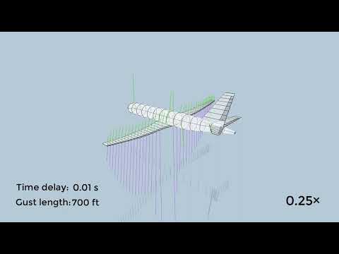
• FlexiFlightVis 0.2 (optional; for visualization): https://github.com/iff-gsc/FlexiFlightVis

Demo

• Initialize the simulation model:
  1. Open MATLAB
  2. Navigate to the project folder and then to the subfolder demo

     cd('demo')
     

  3. Run the initialization script init_flexible_unsteady_indi (Click Change Folder or Add to Path if requested.).

     init_flexible_unsteady_indi
     

• Run the Simulink simulation:
  1. The Simulink model sim_flexible_unsteady_indi should already open during the initialization.
  2. Run the Simulink model.
  3. Several signals are logged in the Scopes and Wing bending moments subsystems.
• Run FlexiFlightVis to see what happens.

Dissertation Results (Data)

All diagrams of the dissertation are provided as TikZ files and can be downloaded in the release area. There is a LaTeX example 0_latex_example.tex in which a TikZ figure is integrated. And there is also the corresponding PDF file 0_latex_example.pdf.

Reproduce Dissertation Results

The diagrams of the dissertation (TikZ files) can be reproduced by running the corresponding simulation. There is a MATLAB script for each figure in the plot_results folder. The table below shows which scripts can be used to create which diagrams.

Figure	Filename	Note
2.1	plot_block_diagram_pics.m
2.9	plot_fuselage.m
2.12	plot_gusts.m
2.13	plot_turbulence_response_delay.m
3.7	plot_actuator_boost_example.m
3.8	plot_booster_avoid_noise.m
3.9	plot_booster_avoid_noise
5.1b	plot_mass_distribution.m
5.2a	plot_wing_definition.m
5.2b	plot_control_effectiveness.m
5.4	plot_eigenmodes.m
5.5	plot_eig.m
5.8a	plot_wrbm_mode_contributions.m
5.8b	plot_wrbm_mode_contributions_gusts.m
6.1	plot_gust_response_cntrl_var.m
6.2	plot_gust_response_cntrl_var.m
6.3	plot_control_allocation.m
6.4	plot_gust_response.m
6.5	plot_gust_response_delay.m
6.7	plot_gust_response_control_inputs.m
6.8	plot_gust_response_delay_gain.m
6.10	plot_gust_envelope_delay_rate_limit.m	In line 66: cntrl_var = 2;
6.11	plot_gust_envelope_delay_rate_limit.m	In line 66: cntrl_var = 2;
6.12	plot_gust_envelope_delay_rate_limit.m	In line 66: cntrl_var = 2;
6.13	plot_gust_envelope_delay_rate_limit.m	In line 66: cntrl_var = 1;
6.14	plot_gust_envelope_delay_rate_limit.m	In line 66: cntrl_var = 1;
6.15	plot_gust_envelope_delay_rate_limit.m	In line 66: cntrl_var = 1;
6.16	plot_turbulence_response_delay.m
6.17	plot_turbulence_response_delay.m
6.18	plot_gust_response_robust_servo.m
6.19	plot_gust_response_robust_delay.m
6.20	plot_gust_response_robust_cntrl_effect.m
6.21	plot_gust_response_failure
6.22	plot_gust_response_delay_stall.m
6.23	plot_gust_response_delay_stall.m
6.24	plot_gust_response_delay_stall.m
6.25	plot_gust_response_delay_stall.m
A.2	plot_gust_response_cntrl_var.m
A.3	plot_gust_response_cntrl_var.m
A.4	plot_gust_envelope_delay_rate_limit.m	In line 66: cntrl_var = 4;
A.5	plot_gust_envelope_delay_rate_limit.m	In line 66: cntrl_var = 4;
A.6	plot_gust_envelope_delay_rate_limit.m	In line 66: cntrl_var = 4;
A.7	plot_gust_envelope_delay_rate_limit.m	In line 66: cntrl_var = -1;
A.8	plot_gust_envelope_delay_rate_limit.m	In line 66: cntrl_var = -1;
A.9	plot_gust_envelope_delay_rate_limit.m	In line 66: cntrl_var = -1;
A.10	plot_gust_envelope_delay_rate_limit.m	In line 66: cntrl_var = 0;
A.11	plot_gust_envelope_delay_rate_limit.m	In line 66: cntrl_var = 0;
A.12	plot_gust_envelope_delay_rate_limit.m	In line 66: cntrl_var = 0;
A.13	plot_gust_envelope_delay_rate_limit.m	In line 66: cntrl_var = 5;
A.14	plot_gust_envelope_delay_rate_limit.m	In line 66: cntrl_var = 5;
A.15	plot_gust_envelope_delay_rate_limit.m	In line 66: cntrl_var = 5;
A.16	plot_gust_envelope_delay_rate_limit.m	In line 66: cntrl_var = 6;
A.17	plot_gust_envelope_delay_rate_limit.m	In line 66: cntrl_var = 6;
A.18	plot_gust_envelope_delay_rate_limit.m	In line 66: cntrl_var = 6;
A.19	plot_gust_response_delay_stall.m	Specify operating point in line 13-16
A.20	plot_gust_response_delay_stall.m	Specify operating point in line 13-16
A.21	plot_gust_response_delay_stall.m	Specify operating point in line 13-16

After the simulation, figures are created which can be exported to TikZ files in the folder results_export.

The plot scripts mostly consist of an initialization of the parameters with trim calculation, simulations, the creation of the figures and the export to a TikZ file. The export to a TikZ file is deactivated by default and can be activated by setting is_tikz_export_desired = true. The trim calculation takes quite a long time. Since the same trim point is often used in different plot scripts, you can often skip the initialization with trim calculation after it has been executed for the first time. In addition, the very first trim calculation takes a very long time because the Simulink model has to be compiled. FlexiFlightVis can be used for visualization during the simulations.

Information about the aeroelastic flight dynamics model can be found in this repository: https://github.com/iff-gsc/SE2A_Aviation_2023