Implementation of various Deep Q-Network (DQN) variants for the state and image inputs of the CartPole-v1 environment. This project was a part of the Fall 2021 Reinforcement Learning course (CS 5180) at Northeastern University.
This project aims to implement and analyze some of the most popular variants of DQN by testing them on image and numerical inputs from the OpenAI-Gym implementation of the Cartpole environment.
For this project, Cartpole-v1 was used, which has a maximum episode length of 500 steps with a maximum reward of 475. A state in this environment consists of 4 features - cart position, cart velocity, pole's angle to the cart and how fast the pole is falling. OpenAI Gym also allows us to render this environment as an image, which could also be used to train a model rather than using the numerical features.
The following DQN Variants are implemented:
After a lot of experiments, the following hyperparameter combination produced the best test results.
| Parameters | DQN | Double DQN | Dueling DQN | NoisyNet DQN |
|---|---|---|---|---|
| Discount factor | 0.99 | 0.99 | 0.99 | 0.99 |
| 1 - 0.05 | 1 - 0.05 | 1 - 0.05 | - | |
| 0.99963 | 0.99963 | 0.99970 | - | |
| Replay Size | 200,000 | 200,000 | 200,000 | 200,000 |
| Batch Size | 256 | 256 | 256 | 256 |
| Target Update Steps | 10,000 | 10,000 | 10,000 | 3,000 |
| Learning Rate | 0.001 | 0.001 | 0.001 | 0.001 |
| Learning Rate Decay | 0.9 | 0.9 | 0.9 | 0.9 |
| LR Decay Steps | 10,000 | 10,000 | 10,000 | 10,000 |
| Parameters | DQN | Double DQN | Dueling DQN | NoisyNet DQN |
|---|---|---|---|---|
| Discount factor | 0.99 | 0.99 | 0.99 | 0.99 |
| 1 - 0.05 | 1 - 0.05 | 1 - 0.05 | - | |
| 0.99984 | 0.99984 | 0.99984 | - | |
| Replay Size | 200,000 | 200,000 | 200,000 | 200,000 |
| Batch Size | 256 | 256 | 256 | 256 |
| Target Update Steps | 10,000 | 10,000 | 10,000 | 10,000 |
| Learning Rate | 0.0001 | 0.0001 | 0.0001 | 0.0001 |
| Learning Rate Decay | 0.9 | 0.9 | 0.9 | 0.9 |
| LR Decay Steps | 25,000 | 25,000 | 25,000 | 20,000 |
After all the models were trained, they were tested on 1,000 random initializations of the CartPole environment. Q-Learning and NoisyNet DQN were able to achieve high scores with relatively short amount of training.
The test scores of the best-performing models on state inputs are as follows:
| Algorithm | Avg. Test Episode Length | Num. Training Episodes |
|---|---|---|
| Q-Learning | 500 | 1,422 |
| DQN | 499.24 | 10,000 |
| Double DQN | 497.63 | 10,000 |
| Dueling DQN | 500 | 10,000 |
| NoisyNet DQN | 500 | 2,000 |
The training curves of the above mentioned algorithms were as follows:
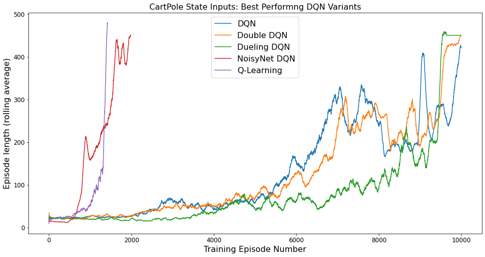
Even with discrete state space and ignoring two features, Q-Learning had the most stable training curves compared to the DQN algorithms. The episode length steadily increased and eventually the policy converged to the optimal policy. The DQN, Double DQN and Dueling DQN algorithms had similar training curves, and all of them took 10,000 episodes to converge or get very close to converging. NoisyNet DQN on the other hand, took only 2,000 episodes to converge to the optimal policy. All of the algorithms were a little unstable when training, with sharp decline in performance every few episodes. But they were able to recover from these performance declines after training for a few more episodes.
The test scores of the best-performing models on the image inputs are as follows:
| Algorithm | Avg. Test Episode Length | Num. Training Episodes |
|---|---|---|
| DQN | 60.53 | 20,000 |
| Double DQN | 38.91 | 20,000 |
| Dueling DQN | 35.04 | 20,000 |
| NoisyNet DQN | 48.24 | 3,000 |
The training curve of the above mentioned algorithms were as follows:
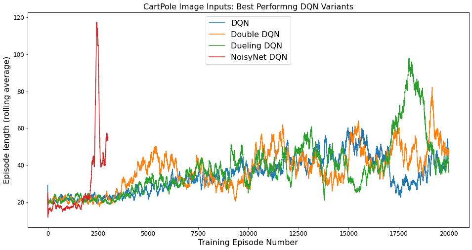
The algorithms with image inputs did not perform nearly as well as the state inputs and overall required longer training times. As can be seen in figure, the training was a lot more unstable than the training for state inputs. After reaching a peak performance, the performance would suddenly drop, resulting in Catastrophic Forgetting. A technique called gradient clipping was also applied, where the gradients are "clipped" to a certain threshold so that a single gradient update does not change the weights by much. However, this also did not seem to help. After running a few experiments, I found that even after increasing the number of training episodes by a few thousand, the network was not be able to recover. To handle catastrophic forgetting, Mnih et al. [1] in the original DQN paper suggested simply to save the parameters that resulted in the best performance.
One of the reasons that the same algorithms do not perform very well on the image inputs as compared to state inputs might be because the convolutional neural network has to first encode the images into a state representation of the environment and this encoding is then used by the fully-connected neural network to get the Q-values. Whereas with the state inputs, this encoding is already derived using intuitive methods.
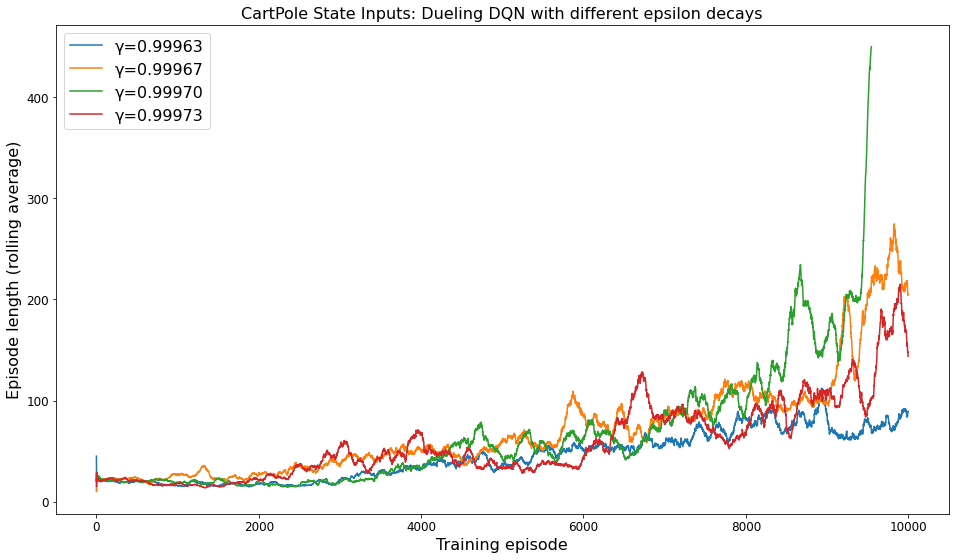
The exponential scheduler for the value of was found to have the most impact on training. Using a scheduler that decays
per time-step (rather than per episode) was very unstable and difficult to tune. Using a scheduler that decays
linearly also did not seem to perform very well. As seen in below figure, increasing the decay rate
by a very small amount led to a significant increase in the performance. The model still shows a slow improvement in episode lengths because there is still a small amount of exploration happening (
). So if we start exploiting without exploring enough, the model might take a really long time to converge (if it doesn't get stuck in a local minima).
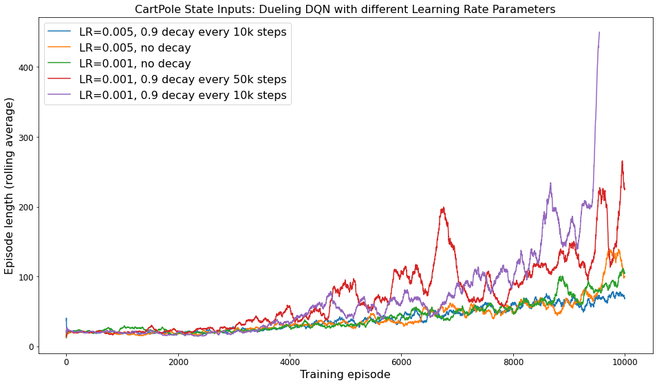
The learning rate was also found to have a significant impact on the performance of the algorithm. Using a constant learning rate throughout the training process resulted in a very slow performance increase over time. Decaying the learning rate slowly (such as the red line in below figure) resulted in a quick performance increase in the beginning, but then a significant drop. This might be because the algorithm reached closer to the optimal policy by taking bigger steps at the beginning, but then it overshot the optima which resulted in a drop in performance. Then when the learning rate eventually decreased, it started getting close to convergence again, but overshot again because the learning rate decay quick enough and the cycle continues.
DQNs are very sensitive to hyperparameters and finding a good combination of hyperparameters has to be a strategic task, because trying every possible combination of them would be extremely time consuming. DQNs that work on images of the environment would be more effective in cases where the environment is very complex, and getting intuitive or simple state representations is difficult. In cases where the state representations are available, image inputs will comparatively perform worse than state inputs.
The DQN algorithms could have performed a lot better with some more hyperparameter search and increasing the number of training episodes. Specifically, using a learning rate scheduler like ReduceLRonPlateau that decays the learning rate only when the performance does not improve over time and starting the decay process near the end of exploration might be useful in increasing the performance of the DQN algorithms.
[1] Mnih Et al.Human-level control through deep reinforcement learning: https://www.nature.com/articles/nature14236
[2] Deep Reinforcement Learning with Double Q-Learning: https://arxiv.org/pdf/1509.06461.pdf
[3] Dueling Network Architectures for Deep Reinforcement Learning: https://arxiv.org/abs/1511.06581
[4] Noisy Networks for Exploration: https://arxiv.org/pdf/1706.10295.pdf