This study investigates the application of Graph Neural Networks (GNN) in electrical power systems, specifically for Power Flow calculation. It compares the performance of GNNs against traditional Neural Networks at equivalent model complexity, with the central research question being: does incorporating data topology improve model accuracy?
This project is my master's thesis at Eindhoven University of Technology. The implementation uses the PyTorch Geometric framework in Jupyter Notebook. The following sections outline the key ideas behind the thesis.
Recent advances in neural networks have introduced new opportunities to incorporate graph topology into machine learning models through a framework known as Graph Neural Networks (GNNs). In power systems, an electrical grid can naturally be represented as a graph with high-dimensional features and strong interdependencies between buses. This idea offers a promising direction for improving machine learning approaches in power system analysis.
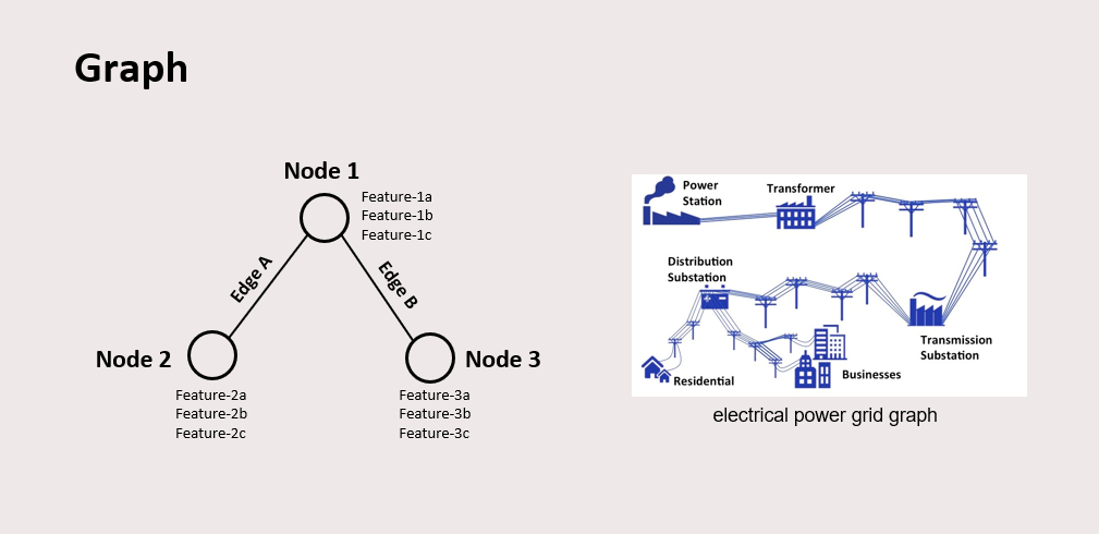
A graph is a data structure composed of nodes and edges, where nodes represent entities and edges represent the connections between them. Graphs are a natural representation for much of the world's data, including proteins, social networks, and electrical power grids.
In a power grid, buses correspond to nodes and transmission lines correspond to edges. Node features include voltage magnitude (V), voltage angle (δ), active power (P), and reactive power (Q), while edge features may include line current (I) and line resistance (R).
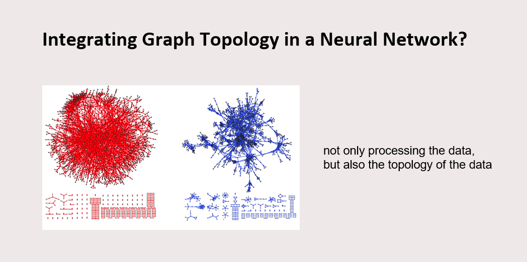
Traditional neural network models such as Multi-Layer Perceptrons (MLP) process only the raw content of data, without considering its structural relationships. GNNs extend this by also leveraging the topology of the data. For example, when applied to protein graphs, a GNN can exploit both the individual molecular properties and the overall structural configuration of the protein, information that a standard MLP would ignore.

In a power grid, buses are classified as slack buses, PV buses, or PQ buses. Each bus type has a distinct set of known and unknown electrical variables. For instance, a PQ bus has known active power (P) and reactive power (Q), but unknown voltage magnitude (V) and voltage angle (δ).
Power Flow (PF) analysis commonly used to solve the unknown variables using electrical equations derived from the known inputs. A GNN-based Power Flow model replaces this numerical solver with a machine learning model that predicts the unknown variables from the known ones.
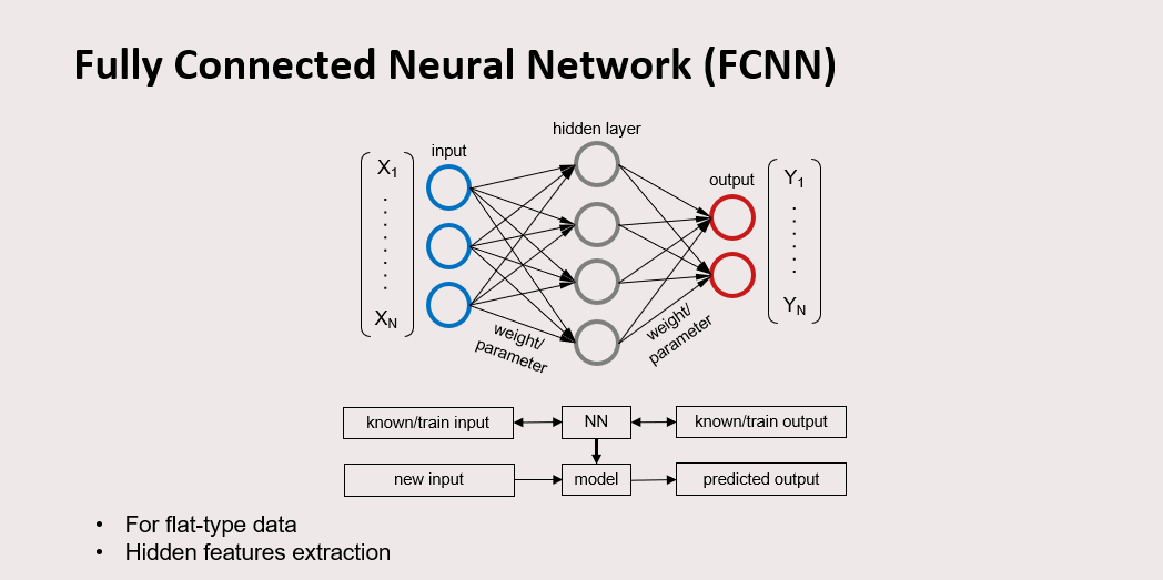
A Fully Connected Neural Network (FCNN) is a supervised machine learning model that learns a mapping between known inputs and outputs. Each connection between nodes represents a trainable weight parameter, which is adjusted iteratively during training.
The model computes predictions by propagating inputs forward through these weighted connections, where each node value is multiplied by its corresponding weight parameter and transformed through successive layers to produce the predicted output, which is then compared with the ground-truth output. The discrepancy between the predicted output and the ground truth is quantified by a loss function, typically cross-entropy for classification or mean squared error for regression. The model is optimized over multiple iterations until it achieves sufficient predictive accuracy. Once trained, it can generalize to unseen inputs. FCNNs are designed for flat, tabular data and perform feature extraction through their hidden layers.
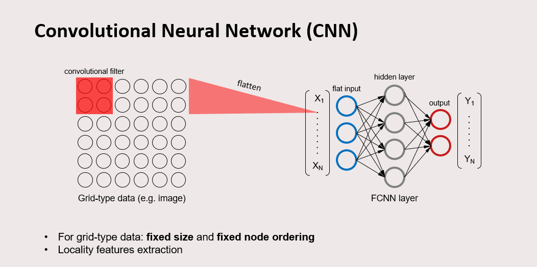
Convolutional Neural Networks (CNN) are designed for grid-structured data: data with a fixed size and a consistent node ordering. A digital image is a canonical example: it consists of pixels arranged in fixed rows and columns with a well-defined spatial order. A CNN applies convolutional filters to the input, flattens the resulting feature maps into a one-dimensional vector, and passes it through a fully connected layer. The convolutional operation specifically exploits the local spatial structure inherent in grid-type data.
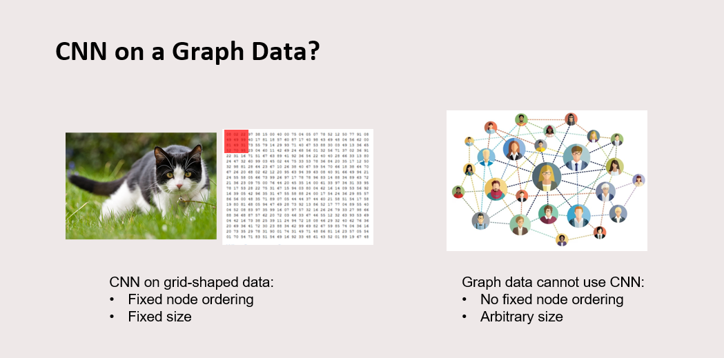
A natural question arises: can CNN be applied to graph-structured data? The answer is no. CNNs require data with a fixed grid structure and consistent node ordering, such as images, whereas graph data has no inherent node ordering. A different mechanism is needed to apply convolution-like operations to graph data, and this is precisely the problem that GNNs are designed to solve.

The core mechanism of GNN is message passing: a process by which each node aggregates information from its neighboring nodes. For example, node 4 receives messages from nodes 1, 5, and 6, as well as from its own previous state. This aggregation occurs across all nodes simultaneously in a single GNN layer. The aggregated messages are summed, multiplied by a trainable weight matrix W, and passed through a non-linear activation function to produce the input for the next layer. But how to implement this mathematically?

This message passing operation can be implemented using the adjacency matrix A, which encodes the connectivity of the graph. For node 4, whose neighbors are nodes 1, 4, 5, and 6, the corresponding row in A is assigned a value of 1 in those columns and 0 elsewhere. Multiplying this row by the node feature matrix X performs a summation over the features of all neighboring nodes, effectively implementing a simple summation message passing.

Graph Convolutional Network (GCN) is a more advanced variant of GNN. The key distinction is that GCN uses averaging rather than summation for message aggregation. This is achieved by preprocessing the adjacency matrix A with the inverse of the degree matrix D, where D encodes the number of neighbors for each node. For instance, since node 4 has 4 neighbors, its row is divided by 4, yielding an average over its neighbors' features. The dimensions of the trainable weight matrix W determine the number of features extracted in each layer.
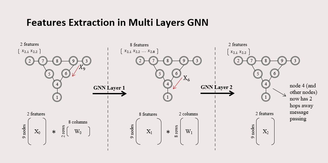
This diagram illustrates hidden feature extraction in a multi-layer GNN applied to a 9-node graph. Each node begins with 2 features. In the first GNN layer, the node features are transformed by weight matrix W0 (2×8), expanding each node's representation to 8 features. The second layer applies weight matrix W1 (8×2), compressing the representation back to 2 features per node.
Notably, node 4 in the final state has indirectly received information from node 9 via node 6, demonstrating that a 2-layer GNN achieves 2-hop message passing, aggregating information from nodes up to two edges away.

Analogous to CNN, GNN layers can be stacked as a component within a broader deep learning architecture. The output of the GNN layers can be flattened and passed into a fully connected layer for final prediction.
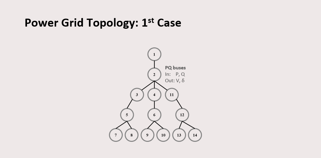
The first graph topology used in this study consists of 14 nodes, where each node represents a PQ bus.

The second graph topology extends the first by introducing loops of varying sizes: small, medium, and large. This variant was designed to evaluate the effect of graph topology complexity, i.e. the presence of cycles, on GNN predictive performance.

Three model architectures were designed for comparison. Model 1 consists of two traditional fully connected layers. Model 2 replaces the first fully connected layer with a single GNN layer. Model 3 uses two GNN layers (equivalent to 2-hop message passing) followed by a fully connected output layer.
All three models were designed to have approximately 2600 trainable parameters to ensure a fair comparison at equivalent model complexity. Detailed hyperparameter configurations are shown in the figure.

The dataset was generated using DIgSILENT PowerFactory 2020. A total of 102 datasets were produced, each containing 2000 data points. Of these, 1 dataset was used for training, 1 for validation, and the remaining 100 for testing.

Each dataset contains 2000 data points. Each data point is structured as a matrix of 14 rows, one per bus node, where each node has 2 input features and 2 output features. When used with fully connected networks, this matrix must first be flattened into a one-dimensional vector.
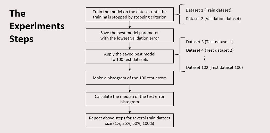
The figure above summarizes the experimental steps followed in this study. The complete results and analysis can be found in the full report here: