Workshop: Setting up, Operation Analitycs, Algorithms + Machine-Learnig, Deployment and BigData with Amazon AWS and EMR (Elastic Map Reduce)

This workshop was held for the working sessions with the company Predictiva. The workshop covers all phases of working with Amazon's BigData platform, including:
- Setting up the initial environment for AWS (Amazon Web Services) and EMR (ElasticMapReduce),
- Creating clusters with Spark, Hadoop and multiple configurations (yarn),
- Working with Steps on EMR,
- Executing experiments and algorithms with Python, Scala and SparkR on EMR (interactive and standalone),
- MachineLearning and DataMining with EMR Cluster,
- Basics with SparkStreaming for real time data analisys
- Working with MongoDB interconecting EC2 (ElasticCloud) nodes,
- and more (see TOC).

- Setting up AWS
- Creating a simple Spark Cluster
- Starting interactive BigData Analytics
- Submitting BigData applications to the cluster
- Starting with Datasets and SparkDataFrames
- Machine Learning examples
- Data Streaming with Spark
- BigData development environment with Spark and Hadoop
- Starting with MongoDB
- Starting with MongoDB
- Extras
AWS Identity and Access Management (IAM) is a web service that helps you securely control access to AWS resources for your users. You use IAM to control who can use your AWS resources (authentication) and what resources they can use and in what ways (authorization).
- Go to IAM.
- Click on the left Add user.
- Write User name
- In Access Type check:
Programmatic access. It enables an access key ID and secret access key for the AWS API, CLI, SDK, and other development tools. - In Permissions add AdministratorAccess Policy (if this user will be administrator).
- Add to Group of AdministratorAccess
The AWS Command Line Interface (CLI) is a unified tool to manage your AWS services. With just one tool to download and configure, you can control multiple AWS services from the command line and automate them through scripts.
Windows
Download and run the 64-bit Windows installer.
Mac and Linux
Requires Python 2.6.5 or higher. Install using pip:
sudo pip install awscli
Use AWS Access Key ID from Security Credentials Tab of the user and the same to AWS Secret Access Key. If you want to generate a new Access key, you will get a new pair of Access Key ID and Secret Access Key.
Check your REGION NAME here.
After install, configure AWS CLI:
$ aws configure
AWS Access Key ID [None]: XXXXXXXXXXXX
AWS Secret Access Key [None]: YYYYYYYYYYYYY
Default region name [None]: eu-west-1
Default output format [None]:
Try:
aws s3 ls
If it returns without error, AWS CLI is working fine.
Amazon EC2/EMR (and all products) uses public–key cryptography to encrypt and decrypt login information. Public–key cryptography uses a public key to encrypt a piece of data, such as a password, then the recipient uses the private key to decrypt the data. The public and private keys are known as a key pair.
To log in our Cluster or Instance, we must create a key pair, specify the name of the key pair when you launch the instance, and provide the private key when you connect to the instance. Linux instances have no password, and you use a key pair to log in using SSH.
To create a key pair:
- Go to EC2 dashboard and click "Create Key Pair".
After this, PEM file will be downloaded, please store this file in a safe location in your computer.
Set 400 permissions mask to PEM file (to avoid this problem connecting with ssh: [PEM Error](#errors/errors.md#UNPROTECTED PRIVATE KEY FILE)).
chmod 400 /home/manuparra/.ssh/PredictivaIO.pem
Creating a Spark Cluster with the next features:
- emr: 5.4.0 see releases.
- KeyName: Name of the Key Pair generated from EC2/KeyPairs (not the
.pemfile). - Name: Name of the software-sandbox. Here you can add more software bundles.
- m3.xlarge: Flavour of the instances. Types.
- instance-count: Number of instances counting the master (ie. 2 -> 1 master 1 slave).
aws emr create-cluster --name "SparkClusterTest" --release-label emr-5.4.0 --applications Name=Spark --ec2-attributes KeyName=PredictivaIO --instance-type m3.xlarge --instance-count 2 --use-default-roles
after this, you will get Cluster ID in JSON this format:
{
    "ClusterId": "j-26H8B5P1XGYM0"
}
To check the status of the created cluster:
aws emr list-clusters
To check the status of active/terminated or failed Clusters ([--active | --terminated | --failed])
aws emr list-clusters --active
This show the following:
{
    "Clusters": [
        {
            "Status": {
                "Timeline": {
                    "ReadyDateTime": 1490305701.226,
                    "CreationDateTime": 1490305385.744
                },
                "State": "WAITING",
                "StateChangeReason": {
                    "Message": "Cluster ready to run steps."
                }
            },
            "NormalizedInstanceHours": 16,
            "Id": "j-26H8B5P1XGYM0",
            "Name": "Spark cluster"
        }
    ]
}
In this moment the Cluster is WAITING.
Valid cluster states include: STARTING, BOOTSTRAPPING, RUNNING, WAITING, TERMINATING, TERMINATED, and TERMINATED_WITH_ERRORS.
We can see all details about the cluster created:
aws emr list-instances --cluster-id j-26H8B5P1XGYM0
Output is:
{
    "Instances": [
        {
            "Status": {
                "Timeline": {
                    "CreationDateTime": 1490356300.053
                },
                "State": "BOOTSTRAPPING",
                "StateChangeReason": {}
            },
            "Ec2InstanceId": "i-001855d3651ae1054",
            "EbsVolumes": [],
            "PublicDnsName": "ec2-54-229-82-137.eu-west-1.compute.amazonaws.com",
            "InstanceType": "m3.xlarge",
            "PrivateDnsName": "ip-172-31-21-212.eu-west-1.compute.internal",
            "Market": "ON_DEMAND",
            "PublicIpAddress": "54.229.82.137",
            "InstanceGroupId": "ig-31OMOWVJ48XGJ",
            "Id": "ci-32ELRJPXEQOR7",
            "PrivateIpAddress": "172.31.21.212"
        },
        {
            "Status": {
                "Timeline": {
                    "CreationDateTime": 1490356300.053
                },
                "State": "BOOTSTRAPPING",
                "StateChangeReason": {}
            },
            "Ec2InstanceId": "i-0ca767cb507dcfd2f",
            "EbsVolumes": [],
            "PublicDnsName": "ec2-54-194-201-167.eu-west-1.compute.amazonaws.com",
            "InstanceType": "m3.xlarge",
            "PrivateDnsName": "ip-172-31-20-141.eu-west-1.compute.internal",
            "Market": "ON_DEMAND",
            "PublicIpAddress": "54.194.201.167",
            "InstanceGroupId": "ig-1JJADD5HFSD8N",
            "Id": "ci-1UNET4ZQB58AD",
            "PrivateIpAddress": "172.31.20.141"
        }
    ]
}
Try the next. If the command cannot connnect, check Security group and add a RULE for SSH :
aws emr ssh --cluster-id j-26H8B5P1XGYM0 --key-pair-file /home/manuparra/.ssh/PredictivaIO.pem
If you have the [PEM Error](#errors/errors.md#UNPROTECTED PRIVATE KEY FILE)) solve it, and try out ssh again.
If the command was fine you will get the next (so, you are connected to the Cluster created):
       __|  __|_  )
       _|  (     /   Amazon Linux AMI
      ___|\___|___|

https://aws.amazon.com/amazon-linux-ami/2016.09-release-notes/
18 package(s) needed for security, out of 41 available
Run "sudo yum update" to apply all updates.

EEEEEEEEEEEEEEEEEEEE MMMMMMMM           MMMMMMMM RRRRRRRRRRRRRRR
E::::::::::::::::::E M:::::::M         M:::::::M R::::::::::::::R
EE:::::EEEEEEEEE:::E M::::::::M       M::::::::M R:::::RRRRRR:::::R
  E::::E       EEEEE M:::::::::M     M:::::::::M RR::::R      R::::R
  E::::E             M::::::M:::M   M:::M::::::M   R:::R      R::::R
  E:::::EEEEEEEEEE   M:::::M M:::M M:::M M:::::M   R:::RRRRRR:::::R
  E::::::::::::::E   M:::::M  M:::M:::M  M:::::M   R:::::::::::RR
  E:::::EEEEEEEEEE   M:::::M   M:::::M   M:::::M   R:::RRRRRR::::R
  E::::E             M:::::M    M:::M    M:::::M   R:::R      R::::R
  E::::E       EEEEE M:::::M     MMM     M:::::M   R:::R      R::::R
EE:::::EEEEEEEE::::E M:::::M             M:::::M   R:::R      R::::R
E::::::::::::::::::E M:::::M             M:::::M RR::::R      R::::R
EEEEEEEEEEEEEEEEEEEE MMMMMMM             MMMMMMM RRRRRRR      RRRRRR

[hadoop@ip-172-31-18-31 ~]$
And now you are in the Master Node of your cluster.
Spark supports Scala, Python and R. We can choose to write them as standalone Spark applications, or within an interactive interpreter.
Once logged in you can use three possible interactive development environments that brings the cluster (by default):
We can use pyspark interactive shell:
[hadoop@ip-[redacted] ~]$ pyspark
Working with this sample:
lines=sc.textFile("s3n://datasets-preditiva/500000_ECBDL14_10tst.data")

print lines.count()

print lines.take(10)

lines.saveAsTextFile("s3n://datasets-preditiva/results/10_ECBDL14_10tst.data")

#from pyspark.sql import Row
#parts = lines.map(lambda l: l.split(","))
#table = parts.map(lambda p: (p[0], p[1] , p[2] , p[3] , p[4] , p[5] , p[6] ))
#schemaTable = spark.createDataFrame(table)
#schemaTable.createOrReplaceTempView("mytable")

#print schemaTable.printSchema()
Press CRTL+D to exit or write exit.
[hadoop@ip-[redacted] ~]$ spark-shell
Working with this sample:
val x = sc.textFile("s3n://datasets-preditiva/500000_ECBDL14_10tst.data")
x.take(5)
x.saveAsTextFile("s3n://datasets-preditiva/results/10_ECBDL14_10tst.data")
Press CRTL+D to exit or write exit.
[hadoop@ip-[redacted] ~]$ sparkR
Working with this sample:
data <- textFile(sc, "s3n://datasets-preditiva/500000_ECBDL14_10tst.data")

brief <- take(data,10)

saveAsTextFile(brief,"s3n://datasets-preditiva/results/10_ECBDL14_10tst.data")
Press CRTL+D to exit or write exit.
Use AWS CLI:
aws emr terminate-clusters --cluster-id j-26H8B5P1XGYM0
You can check if the Cluster is terminated:
aws emr list-clusters --terminated
EMR release contains several distributed applications available for installation on your cluster in all-in-one deployment. EMR defines each application as not only the set of the components which comprise that open source project but also a set of associated components which are required for that the application to function.
When you choose to install an application using the console, API, or CLI, Amazon EMR installs and configures this set of components across nodes in your cluster. The following applications are supported for this release:
- Flink
- Ganglia
- Hadoop
- HBase
- Hive
- Mahout
- Spark
- Zeppelin and more.
Add --application Name=XXXX Name=YYYY, ... to AWS CLI creation command:
aws emr create-cluster --name "SparkClusterTest01" --release-label emr-5.4.0 --applications Name=Spark Name=Hadoop Name=Ganglia Name=Zeppelin --ec2-attributes KeyName=PredictivaIO --instance-type m3.xlarge --instance-count 2 --use-default-roles
Try connect with SSH:
aws emr ssh --cluster-id <Cluster ID> --key-pair-file /home/manuparra/.ssh/PredictivaIO.pem
Remember terminate your cluster is you have finished your job:
aws emr terminate-clusters --cluster-id j-26H8B5P1XGYM0
Just add only Name=Spark and Name=Zeppelin :
aws emr create-cluster --name "SparkClusterTest02" --release-label emr-5.4.0 --applications Name=Spark Name=Zeppelin --ec2-attributes KeyName=PredictivaIO --instance-type m3.xlarge --instance-count 2 --use-default-roles
Try connect with SSH:
aws emr ssh --cluster-id <Cluster ID> --key-pair-file /home/manuparra/.ssh/PredictivaIO.pem
<<<<<<< Updated upstream
=======
Stashed changes
You can override the default configurations for applications you install by supplying a configuration object when specifying applications you want installed at cluster creation time.
Sometimes software installed on the cluster probably use a port to comunicate with it.
To add support to aditional software and show the software on external port, we need to create a RULE on Security group.
Security group acts as a virtual firewall that controls the traffic for one or more instances. When you launch an instance, you associate one or more security groups with the instance. You add rules to each security group that allow traffic to or from its associated instances. You can modify the rules for a security group at any time; the new rules are automatically applied to all instances that are associated with the security group. When we decide whether to allow traffic to reach an instance, we evaluate all the rules from all the security groups that are associated with the instance.
To create or to add a new rule, go to Security Groups in the menu EC2 (choose SecurityGroups) and select:
- ElasticMapReduce-master ... (Master group for Elastic MapReduce created on ....) and Edit Rules on INBOUND :
- Add Custom TCP o UDP Rule
- Add the port specific for the software
- Add Source and choose: Anywhere
We create new Cluster with Zeppelin support:
aws emr create-cluster --name "SparkClusterTest" --release-label emr-5.4.0 --applications Name=Spark Name=Hadoop Name=Ganglia Name=Zeppelin --ec2-attributes KeyName=PredictivaIO --instance-type m3.xlarge --instance-count 2 --use-default-roles
After it has been created, check the details of the cluster and get the Public DNS Name:
aws emr list-instances --cluster-id j-XXXXXXXXXX
Check the PublicDNSName :
    ...
    "PublicDnsName": "ec2-54-229-189-0.eu-west-1.compute.amazonaws.com",
    ...
And now, in your browser:
http://ec2-54-229-189-0.eu-west-1.compute.amazonaws.com:8890
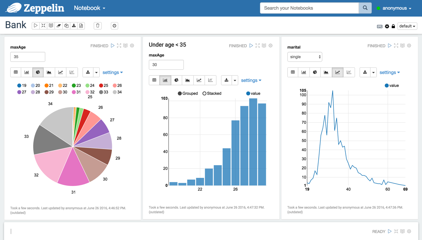
You will see Zeppelin Interactive data analytics web-site of your cluster:
<<<<<<< Updated upstream
=======
Stashed changes
This section describes the methods for submitting work to an AWS EMR cluster. You can submit work to a cluster by adding steps or by interactively submitting Hadoop jobs to the master node. The maximum number of PENDING and ACTIVE steps allowed in a cluster is 256. You can submit jobs interactively to the master node even if you have 256 active steps running on the cluster. You can submit an unlimited number of steps over the lifetime of a long-running cluster, but only 256 steps can be ACTIVE or PENDING at any given time.
The spark-submit script in Spark’s bin directory is used to launch applications on a cluster. It can use all of Spark’s supported cluster managers through a uniform interface so you don’t have to configure your application specially for each one.
<<<<<<< Updated upstream
Connect to your created Cluster via SSH and save the following code in your Cluster home with the name wordcount.py:
Install on created Cluster:
Stashed changes
from __future__ import print_function
from pyspark import SparkContext

<<<<<<< Updated upstream
import sys

if __name__ == "__main__":

    if len(sys.argv) != 3:
        print("Usage: wordcount  ", file=sys.stderr)
        exit(-1)

    sc = SparkContext(appName="WordCount")
    text_file = sc.textFile(sys.argv[1])
=======
Access to python (not ``pyspark``):
>>>>>>> Stashed changes

    counts = text_file.flatMap(lambda line: line.split(" ")).map(lambda word: (word, 1)).reduceByKey(lambda a, b: a + b)

    counts.saveAsTextFile(sys.argv[2])

    sc.stop()
Now execute this command:
spark-submit --deploy-mode cluster --master yarn --num-executors 5 --executor-cores 5 --executor-memory 4g --conf spark.yarn.submit.waitAppCompletion=false wordcount.py s3://datasets-preditiva/inputtext.txt s3://datasets-preditiva/results-wordcount/
Check Memory configuration here.
Note that the property spark.yarn.submit.waitAppCompletion with the step definitions. When this property is set to false, the client submits the application and exits, not waiting for the application to complete. This setting allows you to submit multiple applications to be executed simultaneously by the cluster and is only available in cluster mode.
Connect to your created Cluster via SSH and save the following code in your Cluster home with the name test.R:
args <- commandArgs(trailingOnly = TRUE)

filename <- args[1]
num <- args[2]

data <- textFile(sc, filename)

brief <- take(data,num)

saveAsTextFile(brief,"s3n://datasets-preditiva/results/test-submit-10_ECBDL14_10tst.data")
Now execute this command:
spark-submit --deploy-mode cluster --master yarn --num-executors 5 --executor-cores 5 --executor-memory 4g --conf spark.yarn.submit.waitAppCompletion=false test.R s3://datasets-preditiva/inputtext.txt 10
Now execute this command:
aws emr add-steps --cluster-id j-2L74YHK3V8BCP --steps Type=spark,Name=SparkWordCountApp,Args=[--deploy-mode,cluster,--master,yarn,--conf,spark.yarn.submit.waitAppCompletion=false,--num-executors,5,--executor-cores,5,--executor-memory,8g,s3://code-predictiva/wordcount.py,s3://datasets-preditiva/inputtext.txt,s3://datasets-preditiva/resultswordcount/],ActionOnFailure=CONTINUE
Provides a list of steps for the cluster in reverse order unless you specify stepIds with the request.
aws emr list-steps --cluster-id j-2L74YHK3V8BCP
<<<<<<< Updated upstream
You can cancel steps using the the AWS Management Console, the AWS CLI, or the Amazon EMR API. Only steps that are PENDING can be canceled.
And now, we can use python on spark:
Stashed changes
aws emr cancel-steps --cluster-id j-XXXXXXXXXXXXX --step-ids s-YYYYYYYYYY
A Dataset is a distributed collection of data. Dataset is a new interface added in Spark 1.6 that provides the benefits of RDDs (strong typing, ability to use powerful lambda functions) with the benefits of Spark SQL’s optimized execution engine. A Dataset can be constructed from JVM objects and then manipulated using functional transformations (map, flatMap, filter, etc.). The Dataset API is available in Scala and Java. Python does not have the support for the Dataset API. But due to Python’s dynamic nature, many of the benefits of the Dataset API are already available (i.e. you can access the field of a row by name naturally row.columnName). The case for R is similar.
A DataFrame is a Dataset organized into named columns. It is conceptually equivalent to a table in a relational database or a data frame in R/Python, but with richer optimizations under the hood. DataFrames can be constructed from a wide array of sources such as: structured data files, tables in Hive, external databases, or existing RDDs. The DataFrame API is available in Scala, Java, Python, and R. In Scala and Java, a DataFrame is represented by a Dataset of Rows. In the Scala API, DataFrame is simply a type alias of Dataset[Row]. While, in Java API, users need to use Dataset to represent a DataFrame.

Python:
....

df = spark.read.csv("s3://datasets-preditiva/500000_ECBDL14_10tst.data",header=True, mode="DROPMALFORMED", schema=schema)

df.show()

df.write.save("s3://datasets-preditiva/results-simple/500000_ECBDL14_10tst.data", format="parquet")
R:
df <- read.df("s3://datasets-preditiva/500000_ECBDL14_10tst.data","csv",header = "true", inferSchema = "true");

head(df);

f1andf2 <- select(df, "f1", "f2");

f1andClass <- select(df, "f1", "Class");

write.df(f1andf2, "s3://datasets-preditiva/results-columns-class/", "csv");
write.df(f1andClass, "s3://datasets-preditiva/results-columns-class/", "csv");
Python:
...
df = spark.read.csv("s3://datasets-preditiva/500000_ECBDL14_10tst.data")

# Select columns f1 and f2
df.select("f1","f2")

...
R:
...
df = read.df("s3://datasets-preditiva/500000_ECBDL14_10tst.data","csv",header = "true", inferSchema = "true")

# Select columns f1 and f2
resultDF <- select(df,"f1","f2")

head(resultDF)
...
Python:
...
df = spark.read.csv("s3://datasets-preditiva/500000_ECBDL14_10tst.data")

# Filtering
df.filter(df.f1>0.5 )

...
R:
...
df = read.df("s3://datasets-preditiva/500000_ECBDL14_10tst.data","csv",header = "true", inferSchema = "true")

# Filtering
resultDF <- filter(df,df$f1 > 0.5 & df$f2>0.4)

head(resultDF)
...
Spark SQL supports operating on a variety of data sources through the DataFrame interface. A DataFrame can be operated on using relational transformations and can also be used to create a temporary view. Registering a DataFrame as a temporary view allows you to run SQL queries over its data. This section describes the general methods for loading and saving data using the Spark Data Sources and then goes into specific options that are available for the built-in data sources.
Use createOrReplaceTempView
Python:
...
df = spark.read.csv("s3://datasets-preditiva/500000_ECBDL14_10tst.data")

df.createOrReplaceTempView("tableSQL")

resultDF = spark.sql("SELECT COUNT(*) from tableSQL")
...
R:
...
df = read.df("s3://datasets-preditiva/500000_ECBDL14_10tst.data","csv",header = "true", inferSchema = "true")

createOrReplaceTempView(df,"tableSQL")

resultDF <- sql("SELECT COUNT(*) from tableSQL")

head(resultDF)
...
Python:
# Selecting two columns

df = spark.read.csv("s3://datasets-preditiva/500000_ECBDL14_10tst.data")

df.createOrReplaceTempView("tableSQL")

df.show()

resultDF = spark.sql("SELECT f1, class from tableSQL")
R:
# Selecting two columns

df = read.df("s3://datasets-preditiva/500000_ECBDL14_10tst.data","csv",header = "true", inferSchema = "true")

createOrReplaceTempView(df,"tableSQL")

resultDF <- sql("SELECT f1,class from tableSQL")
Python:
# Selecting two columns and filtering with condition

df = spark.read.csv("s3://datasets-preditiva/500000_ECBDL14_10tst.data")

df.createOrReplaceTempView("tableSQL")

df.show()

resultDF = spark.sql("SELECT f1, class from tableSQL where class='1'")
R:
# Selecting two columns and filtering with condition

df = read.df("s3://datasets-preditiva/500000_ECBDL14_10tst.data","csv",header = "true", inferSchema = "true")

createOrReplaceTempView(df,"tableSQL")

resultDF <- sql("SELECT f1, class from tableSQL where class='1'")
Python:
# Selecting  columns and filtering with multiple conditions

df = spark.read.csv("s3://datasets-preditiva/500000_ECBDL14_10tst.data")

df.createOrReplaceTempView("tableSQL")

df.show()

resultDF = spark.sql("SELECT f1, class from tableSQL where class='1' and f1>0.5 ")
R:
# Selecting  columns and filtering with multiple conditions

df = read.df("s3://datasets-preditiva/500000_ECBDL14_10tst.data","csv",header = "true", inferSchema = "true")

createOrReplaceTempView(df,"tableSQL")

resultDF <- sql("SELECT f1, class from tableSQL where class='1' and f1>0.5")
Python:
df = spark.read.csv("s3://datasets-preditiva/500000_ECBDL14_10tst.data")

df.createOrReplaceTempView("tableSQL")

resultDF = spark.sql("SELECT count(*),class from tableSQL group by class")
R:
# Count the number of elements of the class

df = read.df("s3://datasets-preditiva/500000_ECBDL14_10tst.data","csv",header = "true", inferSchema = "true")

createOrReplaceTempView(df,"tableSQL")

resultDF <- sql("SELECT count(*),class from tableSQL group by class")
Python:
df = spark.read.csv("s3://datasets-preditiva/500000_ECBDL14_10tst.data")

df.createOrReplaceTempView("tableSQL")

resultDF = spark.sql("SELECT SUM(f1),AVG(f3),class from tableSQL group by class")

resultDF.show()
R:
# Count the number of elements of the class

df = read.df("s3://datasets-preditiva/500000_ECBDL14_10tst.data","csv",header = "true", inferSchema = "true")

createOrReplaceTempView(df,"tableSQL")

resultDF <- sql("SELECT SUM(f1),AVG(f3),class from tableSQL group by class")
All functions for SparkSQL aggregation and filtering are defined here.
MachineLearning Lib contains:
- Basic statistics
- summary statistics
- correlations
- stratified sampling
- hypothesis testing
- streaming significance testing
- random data generation
- Classification and regression
- linear models (SVMs, logistic regression, linear regression)
- naive Bayes
- decision trees
- ensembles of trees (Random Forests and Gradient-Boosted Trees)
- isotonic regression
- Collaborative filtering
- alternating least squares (ALS)
- Clustering
- k-means
- Gaussian mixture
- power iteration clustering (PIC)
- latent Dirichlet allocation (LDA)
- bisecting k-means
- streaming k-means
- Dimensionality reduction
- singular value decomposition (SVD)
- principal component analysis (PCA)
- Feature extraction and transformation
- Frequent pattern mining
- FP-growth
- association rules
- PrefixSpan
- Evaluation metrics
- PMML model export
- Optimization (developer)
- stochastic gradient descent
- limited-memory BFGS (L-BFGS)
MLLib guide here
Here are just a few ML methods; All that can be applied is in the previous link.
Examples from http://spark.apache.org/docs/latest/ml-classification-regression.html
Python:
from pyspark.ml.classification import LogisticRegression

# Load training data
training = spark.read.format("libsvm").load("data/mllib/sample_libsvm_data.txt")

lr = LogisticRegression(maxIter=10, regParam=0.3, elasticNetParam=0.8)

# Fit the model
lrModel = lr.fit(training)

# Print the coefficients and intercept for logistic regression
print("Coefficients: " + str(lrModel.coefficients))
print("Intercept: " + str(lrModel.intercept))

# We can also use the multinomial family for binary classification
mlr = LogisticRegression(maxIter=10, regParam=0.3, elasticNetParam=0.8, family="multinomial")

# Fit the model
mlrModel = mlr.fit(training)

# Print the coefficients and intercepts for logistic regression with multinomial family
print("Multinomial coefficients: " + str(mlrModel.coefficientMatrix))
print("Multinomial intercepts: " + str(mlrModel.interceptVector))
R:
# Load training data
df <- read.df("data/mllib/sample_libsvm_data.txt", source = "libsvm")
training <- df
test <- df

# Fit an binomial logistic regression model with spark.logit
model <- spark.logit(training, label ~ features, maxIter = 10, regParam = 0.3, elasticNetParam = 0.8)

# Model summary
summary(model)

# Prediction
predictions <- predict(model, test)
showDF(predictions)
Python:
from pyspark.ml import Pipeline
from pyspark.ml.classification import RandomForestClassifier
from pyspark.ml.feature import IndexToString, StringIndexer, VectorIndexer
from pyspark.ml.evaluation import MulticlassClassificationEvaluator

# Load and parse the data file, converting it to a DataFrame.
data = spark.read.format("libsvm").load("data/mllib/sample_libsvm_data.txt")

# Index labels, adding metadata to the label column.
# Fit on whole dataset to include all labels in index.
labelIndexer = StringIndexer(inputCol="label", outputCol="indexedLabel").fit(data)

# Automatically identify categorical features, and index them.
# Set maxCategories so features with > 4 distinct values are treated as continuous.
featureIndexer =\
    VectorIndexer(inputCol="features", outputCol="indexedFeatures", maxCategories=4).fit(data)

# Split the data into training and test sets (30% held out for testing)
(trainingData, testData) = data.randomSplit([0.7, 0.3])

# Train a RandomForest model.
rf = RandomForestClassifier(labelCol="indexedLabel", featuresCol="indexedFeatures", numTrees=10)

# Convert indexed labels back to original labels.
labelConverter = IndexToString(inputCol="prediction", outputCol="predictedLabel",
                               labels=labelIndexer.labels)

# Chain indexers and forest in a Pipeline
pipeline = Pipeline(stages=[labelIndexer, featureIndexer, rf, labelConverter])

# Train model.  This also runs the indexers.
model = pipeline.fit(trainingData)

# Make predictions.
predictions = model.transform(testData)

# Select example rows to display.
predictions.select("predictedLabel", "label", "features").show(5)

# Select (prediction, true label) and compute test error
evaluator = MulticlassClassificationEvaluator(
    labelCol="indexedLabel", predictionCol="prediction", metricName="accuracy")
accuracy = evaluator.evaluate(predictions)
print("Test Error = %g" % (1.0 - accuracy))

rfModel = model.stages[2]
print(rfModel)  # summary only
R:
# Load training data
df <- read.df("data/mllib/sample_libsvm_data.txt", source = "libsvm")
training <- df
test <- df

# Fit a random forest classification model with spark.randomForest
model <- spark.randomForest(training, label ~ features, "classification", numTrees = 10)

# Model summary
summary(model)

# Prediction
predictions <- predict(model, test)
showDF(predictions)
Python:
from pyspark.ml.regression import GeneralizedLinearRegression

# Load training data
dataset = spark.read.format("libsvm")\
    .load("data/mllib/sample_linear_regression_data.txt")

glr = GeneralizedLinearRegression(family="gaussian", link="identity", maxIter=10, regParam=0.3)

# Fit the model
model = glr.fit(dataset)

# Print the coefficients and intercept for generalized linear regression model
print("Coefficients: " + str(model.coefficients))
print("Intercept: " + str(model.intercept))

# Summarize the model over the training set and print out some metrics
summary = model.summary
print("Coefficient Standard Errors: " + str(summary.coefficientStandardErrors))
print("T Values: " + str(summary.tValues))
print("P Values: " + str(summary.pValues))
print("Dispersion: " + str(summary.dispersion))
print("Null Deviance: " + str(summary.nullDeviance))
print("Residual Degree Of Freedom Null: " + str(summary.residualDegreeOfFreedomNull))
print("Deviance: " + str(summary.deviance))
print("Residual Degree Of Freedom: " + str(summary.residualDegreeOfFreedom))
print("AIC: " + str(summary.aic))
print("Deviance Residuals: ")
summary.residuals().show()
R:
irisDF <- suppressWarnings(createDataFrame(iris))
# Fit a generalized linear model of family "gaussian" with spark.glm
gaussianDF <- irisDF
gaussianTestDF <- irisDF
gaussianGLM <- spark.glm(gaussianDF, Sepal_Length ~ Sepal_Width + Species, family = "gaussian")

# Model summary
summary(gaussianGLM)

# Prediction
gaussianPredictions <- predict(gaussianGLM, gaussianTestDF)
showDF(gaussianPredictions)

# Fit a generalized linear model with glm (R-compliant)
gaussianGLM2 <- glm(Sepal_Length ~ Sepal_Width + Species, gaussianDF, family = "gaussian")
summary(gaussianGLM2)

# Fit a generalized linear model of family "binomial" with spark.glm
# Note: Filter out "setosa" from label column (two labels left) to match "binomial" family.
binomialDF <- filter(irisDF, irisDF$Species != "setosa")
binomialTestDF <- binomialDF
binomialGLM <- spark.glm(binomialDF, Species ~ Sepal_Length + Sepal_Width, family = "binomial")

# Model summary
summary(binomialGLM)

# Prediction
binomialPredictions <- predict(binomialGLM, binomialTestDF)
showDF(binomialPredictions)
To run this on your local machine, you need to first run a Netcat server
$ nc -lk 9999
and then run the example
$ spark-submit network_wordcount.py localhost 9999
from __future__ import print_function

import sys

from pyspark import SparkContext
from pyspark.streaming import StreamingContext

if __name__ == "__main__":
    if len(sys.argv) != 3:
        print("Usage: network_wordcount.py <hostname> <port>", file=sys.stderr)
        exit(-1)


    # Create a local StreamingContext with two working thread and batch interval of 1 second
    sc = SparkContext(appName="PythonStreamingNetworkWordCount")
    ssc = StreamingContext(sc, 1)


    # Create a DStream that will connect to hostname:port, like localhost:9999
    lines = ssc.socketTextStream(sys.argv[1], int(sys.argv[2]))

    # Split each line into words etc,
    counts = lines.flatMap(lambda line: line.split(" "))\
                  .map(lambda word: (word, 1))\
                  .reduceByKey(lambda a, b: a+b)

    # Print the first ten elements of each RDD generated in this DStream to the console
    counts.pprint()

    ssc.start() # Start the computation
    ssc.awaitTermination() # Wait for the computation to terminate
After a context is defined, you have to do the following:
- Define the input sources by creating input DStreams.
- Define the streaming computations by applying transformation and output operations to DStreams.
- Start receiving data and processing it using streamingContext.start().
- Wait for the processing to be stopped (manually or due to any error) using streamingContext.awaitTermination().
- The processing can be manually stopped using streamingContext.stop().
Points to remember:
- Once a context has been started, no new streaming computations can be set up or added to it.
- Once a context has been stopped, it cannot be restarted.
- Only one StreamingContext can be active in a JVM at the same time. stop() on StreamingContext also stops the SparkContext. To stop only the StreamingContext, set the optional parameter of stop() called stopSparkContext to false.
- A SparkContext can be re-used to create multiple StreamingContexts, as long as the previous StreamingContext is stopped (without stopping the SparkContext) before the next StreamingContext is created.
Spark Streaming provides two categories of built-in streaming sources.
- Basic sources: Sources directly available in the StreamingContext API. Examples: file systems, and socket connections.
- Advanced sources: Sources like Kafka, Flume, Kinesis, etc. are available through extra utility classes.
To run this on your local machine, you need to first run a Netcat server
$ nc -lk 9999
and then run the example
$ bin/spark-submit examples/src/main/python/streaming/sql_network_wordcount.py localhost 9999
from __future__ import print_function

import sys

from pyspark import SparkContext
from pyspark.streaming import StreamingContext
from pyspark.sql import Row, SparkSession


def getSparkSessionInstance(sparkConf):
    if ('sparkSessionSingletonInstance' not in globals()):
        globals()['sparkSessionSingletonInstance'] = SparkSession\
            .builder\
            .config(conf=sparkConf)\
            .getOrCreate()
    return globals()['sparkSessionSingletonInstance']


if __name__ == "__main__":
    if len(sys.argv) != 3:
        print("Usage: sql_network_wordcount.py <hostname> <port> ", file=sys.stderr)
        exit(-1)
    host, port = sys.argv[1:]
    sc = SparkContext(appName="PythonSqlNetworkWordCount")
    ssc = StreamingContext(sc, 1)

    # Create a socket stream on target ip:port and count the
    # words in input stream of \n delimited text (eg. generated by 'nc')
    lines = ssc.socketTextStream(host, int(port))
    words = lines.flatMap(lambda line: line.split(" "))

    # Convert RDDs of the words DStream to DataFrame and run SQL query
    def process(time, rdd):
        print("========= %s =========" % str(time))

        try:
            # Get the singleton instance of SparkSession
            spark = getSparkSessionInstance(rdd.context.getConf())

            # Convert RDD[String] to RDD[Row] to DataFrame
            rowRdd = rdd.map(lambda w: Row(word=w))
            wordsDataFrame = spark.createDataFrame(rowRdd)

            # Creates a temporary view using the DataFrame.
            wordsDataFrame.createOrReplaceTempView("words")

            # Do word count on table using SQL and print it
            wordCountsDataFrame = \
                spark.sql("select word, count(*) as total from words group by word")
            wordCountsDataFrame.show()
        except:
            pass

    words.foreachRDD(process)
    ssc.start()
    ssc.awaitTermination()
Check this documentation.
from pyspark.sql import SparkSession
from pyspark.sql.functions import explode
from pyspark.sql.functions import split

spark = SparkSession \
    .builder \
    .appName("StructuredNetworkWordCount") \
    .getOrCreate()

# Create DataFrame representing the stream of input lines from connection to localhost:9999
lines = spark \
    .readStream \
    .format("socket") \
    .option("host", "localhost") \
    .option("port", 9999) \
    .load()

# Split the lines into words
words = lines.select(
   explode(
       split(lines.value, " ")
   ).alias("word")
)

# Generate running word count
wordCounts = words.groupBy("word").count()

# Start running the query that prints the running counts to the console
query = wordCounts \
    .writeStream \
    .outputMode("complete") \
    .format("console") \
    .start()

query.awaitTermination()
Streaming DataFrames can be created through the DataStreamReader interface (Scala/Java/Python docs) returned by SparkSession.readStream(). Similar to the read interface for creating static DataFrame, you can specify the details of the source – data format, schema, options, etc.
Data Sources
In Spark 2.0, there are a few built-in sources.
-
File source - Reads files written in a directory as a stream of data. Supported file formats are text, csv, json, parquet. See the docs of the DataStreamReader interface for a more up-to-date list, and supported options for each file format. Note that the files must be atomically placed in the given directory, which in most file systems, can be achieved by file move operations.
-
Kafka source - Poll data from Kafka. It’s compatible with Kafka broker versions 0.10.0 or higher. See the Kafka Integration Guide for more details.
-
Socket source (for testing) - Reads UTF8 text data from a socket connection. The listening server socket is at the driver. Note that this should be used only for testing as this does not provide end-to-end fault-tolerance guarantees.
Download the virtual machine with the development environment here. (approx: 4 GB)
Credentials to the Virtual Machine are:
- User: root
- Key: sparkR
- VIRTUALBOX installed, available at: https://www.virtualbox.org/wiki/Downloads
- At least 2GB of RAM for the Virtual Machine (datasets must be less than 2GB).
- PC must be 64bit and at least 4GB of RAM (2GB for MVirtual and another 2GB for PC)
- Compatible with Windows, Mac OSX and Linux
Virtual Machine exposes a few ports:
- shh on 22000
- Jupyter notebooks on 25980 (for Spark Python development).
- RStudio on 8787 (for SparkR develpment)
Connecting with SSH:
ssh -p 22000 root@localhost
Connecting with Jupyter Notebooks :
http://localhost:25980
Connecting with RStudio:
http://localhost:8787
Read https://docs.mongodb.com/manual/tutorial/install-mongodb-on-amazon/
First, install in a EC2 instance MongoDB:
sudo vi /etc/yum.repos.d/mongodb-org.repo
Copy the next code:
[mongodb-org-3.4]
name=MongoDB Repository
baseurl=https://repo.mongodb.org/yum/amazon/2013.03/mongodb-org/3.4/x86_64/
gpgcheck=1
enabled=1
gpgkey=https://www.mongodb.org/static/pgp/server-3.4.asc
and then:
sudo yum update
and:
sudo yum install -y mongodb-org
Start the service:
sudo service mongod start
Download the next dataset on your instance home:
wget http://www.barchartmarketdata.com/data-samples/mstf.csv;
mongoimport --host 172.31.25.15 mstf.csv --type csv --headerline -d marketdata -c minbars
Check if dataset is imported:
mongo
Execute the next:
use marketdata

db.minbars.findOne()
If it returns results, dataset has been imported.
Why I use MongoDB Server on 172.31.30.138? This is the IP of the MasterNode, if you require to connect to EC2 Instance, change the IP as needed and remember add the Rule to Security Groups (Inbound Rule, add port 27017 from Anywhere).
How do I change listening IP on MongoDB?
vi /etc/mongodb.conf
and change bind=127.0.0.1 to your Server IP.
To set MongoDB and make available, mongoDB requiere the package: org.mongodb.spark:mongo-spark-connector_2.10:2.0.0
Check the next using interactive python spark:
pyspark --packages org.mongodb.spark:mongo-spark-connector_2.10:2.0.0 --conf "spark.mongodb.input.uri=mongodb://172.31.30.138/marketdata.minbars" --conf "spark.mongodb.output.uri=mongodb://172.31.30.138/marketdata.minbars"
Load MongoDB --conf Database and Collection (here: /marketdata.minbars --> .):
df = spark.read.format("com.mongodb.spark.sql.DefaultSource").load()
Load MongoDB specific Database:
df = spark.read.format("com.mongodb.spark.sql.DefaultSource").option("uri","mongodb://172.31.30.138/marketdata.minbars").load()
Copy this code in your home with the name mongopython.py:
from __future__ import print_function
from pyspark import SparkContext

import sys

if __name__ == "__main__":

    sc = SparkContext(appName="TestMongoDB")

    df=sc.read.format("com.mongodb.spark.sql.DefaultSource").load()

    print df.printSchema()

    df.write.save("s3://datasets-preditiva/results-simple/mongosaved.csv", format="csv")

    sc.stop()
from pyspark.sql import SparkSession

from __future__ import print_function
from pyspark import SparkContext

import sys

if __name__ == "__main__":

  my_spark = SparkSession.builder.appName("myApp").config("spark.mongodb.input.uri", "mongodb://172.31.19.25/marketdata.minbars").config("spark.mongodb.output.uri", "mongodb://172.31.19.25/marketdata.minbars").getOrCreate()
spark-submit --deploy-mode cluster --master yarn --num-executors 5 --executor-cores 5 --executor-memory 4g --conf spark.yarn.submit.waitAppCompletion=false --conf "spark.mongodb.input.uri=mongodb://172.31.19.25/marketdata.minbars" --conf "spark.mongodb.output.uri=mongodb://172.31.19.25/marketdata.minbars" --packages org.mongodb.spark:mongo-spark-connector_2.10:2.0.0 mongopython.py
MongoDB is an open-source database developed by MongoDB, Inc.
MongoDB stores data in JSON-like documents that can vary in structure. Related information is stored together for fast query access through the MongoDB query language. MongoDB uses dynamic schemas, meaning that you can create records without first defining the structure, such as the fields or the types of their values. You can change the structure of records (which we call documents) simply by adding new fields or deleting existing ones. This data model give you the ability to represent hierarchical relationships, to store arrays, and other more complex structures easily. Documents in a collection need not have an identical set of fields and denormalization of data is common. MongoDB was also designed with high availability and scalability in mind, and includes out-of-the-box replication and auto-sharding.
MongoDB main features:
- Document Oriented Storage − Data is stored in the form of JSON style documents.
- Index on any attribute
- Replication and high availability
- Auto-sharding
- Rich queries
Using Mongo:
- Big Data
- Content Management and Delivery
- Mobile and Social Infrastructure
- User Data Management
- Data Hub
Compared to MySQL:
Many concepts in MySQL have close analogs in MongoDB. Some of the common concepts in each system:
- MySQL -> MongoDB
- Database -> Database
- Table -> Collection
- Row -> Document
- Column -> Field
- Joins -> Embedded documents, linking
Query Language:
From MySQL:
INSERT INTO users (user_id, age, status)
VALUES ('bcd001', 45, 'A');
To MongoDB:
db.users.insert({
  user_id: 'bcd001',
  age: 45,
  status: 'A'
});
From MySQL:
SELECT * FROM users
To MongoDB:
db.users.find()
From MySQL:
UPDATE users SET status = 'C'
WHERE age > 25
To MongoDB:
db.users.update(
  { age: { $gt: 25 } },
  { $set: { status: 'C' } },
  { multi: true }
)
MongoDB stores data records as BSON documents.
BSON is a binary representation of JSON documents, it contains more data types than JSON.

MongoDB documents are composed of field-and-value pairs and have the following structure:
{
   field1: value1,
   field2: value2,
   field3: value3,
   ...
   fieldN: valueN
}
Example of document:
var mydoc = {
               _id: ObjectId("5099803df3f4948bd2f98391"),
               name:
                    {
                     first: "Alan",
                     last: "Turing"
                    },
               birth: new Date('Jun 23, 1912'),
               death: new Date('Jun 07, 1954'),
               contribs: [
                            "Turing machine",
                            "Turing test",
                            "Turingery" ],
               views : NumberLong(1250000)
            }
To specify or access a field of an document: use dot notation
mydoc.name.first
Documents allow embedded documents embedded documents embedded documents ...:
{
   ...
   name: { first: "Alan", last: "Turing" },
   contact: {
            phone: {
                    model: {
                        brand: "LG",
                        screen: {'maxres': "1200x800"}
                    },
                    type: "cell",
                    number: "111-222-3333" } },
   ...
}
The maximum BSON document size is 16 megabytes!.
- String − This is the most commonly used datatype to store the data.
- Integer − This type is used to store a numerical value.
- Boolean − This type is used to store a boolean (true/ false) value.
- Double − This type is used to store floating point values.
- Min/ Max keys − This type is used to compare a value against the lowest and highest BSON elements.
- Arrays − This type is used to store arrays or list or multiple values into one key.
- Timestamp − ctimestamp. This can be handy for recording when a document has been modified or added.
- Object − This datatype is used for embedded documents.
- Null − This type is used to store a Null value.
- Symbol − This datatype is used identically to a string; however, it's generally reserved for languages that use a specific symbol type.
- Date − This datatype is used to store the current date or time in UNIX time format. You can specify your own date time by creating object of Date and passing day, month, year into it.
- Object ID − This datatype is used to store the document’s ID.
- Binary data − This datatype is used to store binary data.
- Code − This datatype is used to store JavaScript code into the document.
- Regular expression − This datatype is used to store regular expression.
sudo yum install mongodb-org
After install:
sudo systemctl start mongod
Log and connect to our system with:
First of all, check that you have access to the mongo tools system, try this command:
mongo + tab
it will show:
mongo         mongodump     mongoexport   mongofiles
mongoimport   mongooplog    mongoperf     mongorestore  mongostat     mongotop
The default port for mongodb and mongos instances is 27017. You can change this port with port or --port when connect.
Write:
mongo
It will connect with defaults parameters: localhost , port: 27017 and database: test
MongoDB shell version: 2.6.12
connecting to: test
>
Exit using CTRL+C or exit
Each user have an account on mongodb service. To connect:
mongo localhost:27017/manuparra -p
It will us password.
mongo localhost:27017/manuparra -p mipasss
MongoDB service is running locally in Docker systems, so, if you connect from docker containers or Virtual Machines, you must to use local docker system IP:
mongo 192.168.10.30:27017/manuparra -p mipasss
The command will create a new database if it doesn't exist, otherwise it will return the existing database.
> use manuparra:
Now you are using manuparra database.
If you want to kwnow what database are you using:
> db
The ```command db.dropDatabase()`` is used to drop a existing database.
DO NOT USE THIS COMMAND, WARNING:
db.dropDatabase()
To kwnow the size of databases:
show dbs
Basic syntax of createCollection() command is as follows:
db.createCollection(name, options)
where options is Optional and specify options about memory size and indexing.
Remember that firstly mongodb needs to kwnow what is the Database where it will create the Collection. Use show dbs and then use <your database>.
use manuparra;
And then create the collection:
db.createCollection("MyFirstCollection")
When created check:
show collections
In MongoDB, you don't need to create the collection. MongoDB creates collection automatically, when you insert some document:
db.MySecondCollection.insert({"name" : "Manuel Parra"})
You have new collections created:
show collections
To remove a collection from the database:
db.MySecondCollection.drop();
To insert data into MongoDB collection, you need to use MongoDB's insert() or save() method.
> db.MyFirstCollection.insert(<document>);
Example of document: place
{
     "bounding_box":
    {
        "coordinates":
        [[
                [-77.119759,38.791645],
                [-76.909393,38.791645],
                [-76.909393,38.995548],
                [-77.119759,38.995548]
        ]],
        "type":"Polygon"
    },
     "country":"United States",
     "country_code":"US",
     "likes":2392842343,
     "full_name":"Washington, DC",
     "id":"01fbe706f872cb32",
     "name":"Washington",
     "place_type":"city",
     "url": "http://api.twitter.com/1/geo/id/01fbe706f872cb32.json"
}
To insert:
db.MyFirstCollection.insert(
{
     "bounding_box":
      {
        "coordinates":
        [[
                [-77.119759,38.791645],
                [-76.909393,38.791645],
                [-76.909393,38.995548],
                [-77.119759,38.995548]
        ]],
        "type":"Polygon"
      },
     "country":"United States",
     "country_code":"US",
     "likes":2392842343,
     "full_name":"Washington, DC",
     "id":"01fbe706f872cb32",
     "name":"Washington",
     "place_type":"city",
     "url": "http://api.twitter.com/1/geo/id/01fbe706f872cb32.json"
}
);
Check if document is stored:
> db.MyFirstCollection.find();
Add multiple documents:
    var places= [
        {
         "bounding_box":
          {
            "coordinates":
            [[
                    [-77.119759,38.791645],
                    [-76.909393,38.791645],
                    [-76.909393,38.995548],
                    [-77.119759,38.995548]
            ]],
            "type":"Polygon"
          },
         "country":"United States",
         "country_code":"US",
         "likes":2392842343,
         "full_name":"Washington, DC",
         "id":"01fbe706f872cb32",
         "name":"Washington",
         "place_type":"city",
         "url": "http://api.twitter.com/1/geo/id/01fbe706f872cb32.json"
    },
    {
         "bounding_box":
          {
            "coordinates":
            [[
                    [-7.119759,33.791645],
                    [-7.909393,34.791645],
                    [-7.909393,32.995548],
                    [-7.119759,34.995548]
            ]],
            "type":"Polygon"
          },
         "country":"Spain",
         "country_code":"US",
         "likes":2334244,
         "full_name":"Madrid",
         "id":"01fbe706f872cb32",
         "name":"Madrid",
         "place_type":"city",
         "url": "http://api.twitter.com/1/geo/id/01fbe706f87333e.json"
    }
    ]
and:
db.MyFirstCollection.insert(places)
In the inserted document, if we don't specify the _id parameter, then MongoDB assigns a unique ObjectId for this document.
You can override value _id, using your own _id.
Two methods to save/insert:
db.MyFirstCollection.save({username:"myuser",password:"mypasswd"})
db.MyFirstCollection.insert({username:"myuser",password:"mypasswd"})
Differences:
If a document does not exist with the specified
_idvalue, thesave()method performs an insert with the specified fields in the document.
If a document exists with the specified
_id` value, thesave()`` method performs an update, replacing all field in the existing record with the fields from the document.
Show all documents in MyFirstCollection:
> db.MyFirstCollection.find();
Only one document, not all:
> db.MyFirstCollection.findOne();
Counting documents, add .count() to your sentences:
> db.MyFirstCollection.find().count();
Show documentos in pretty mode:
> db.MyFirstCollection.find().pretty()
Selecting or searching by embeded fields, for example bounding_box.type:
...
 "bounding_box":
    {
        "coordinates":
        [[
                [-77.119759,38.791645],
                [-76.909393,38.791645],
                [-76.909393,38.995548],
                [-77.119759,38.995548]
        ]],
        "type":"Polygon"
    },
...
> db.MyFirstCollection.find("bounding_box.type":"Polygon")
Filtering:
Equality {<key>:<value>} db.MyFirstCollection.find({"country":"Spain"}).pretty()
Less Than {<key>:{$lt:<value>}} db.mycol.find({"likes":{$lt:50}}).pretty()
Less Than Equals {<key>:{$lte:<value>}} db.mycol.find({"likes":{$lte:50}}).pretty()
Greater Than {<key>:{$gt:<value>}} db.mycol.find({"likes":{$gt:50}}).pretty()
More: gte Greater than equal, ne Not equal, etc.
AND:
> db.MyFirstCollection.find(
   {
      $and: [
         {key1: value1}, {key2:value2}
      ]
   }
).pretty()
OR:
db.MyFirstCollection.find( { $or: [ {key1: value1}, {key2:value2} ] } ).pretty()
Mixing up :
db.MyFirstCollection.find(
        {"likes": {$gt:10},
         $or:
            [
             {"by": "..."},
             {"title": "..."}
            ]
        }).pretty()
Using regular expresions on fields, for instance to search documents where the name field
name cointais Wash.
db.MyFirstCollection.find({"name": /.*Wash.*/})
Syntax:
> db.MyFirstCollection.update(<selection criteria>, <data to update>)
Example:
db.MyFirstCollection.update(
     { 'place_type':'area'},
     { $set: {'title':'New MongoDB Tutorial'}},
     {multi:true}
    );
IMPORTANT: use multi:true to update all coincedences.
MongoDB's remove() method is used to remove a document from the collection. remove() method accepts two parameters. One is deletion criteria and second is justOne flag.
> db.MyFirstCollection.remove(<criteria>)
Example:
db.MyFirstCollection.remove({'country':'United States'})
Download this dataset in your Docker Home (copy this link: http://samplecsvs.s3.amazonaws.com/SacramentocrimeJanuary2006.csv):
DataSet 7585 rows and 794 KB)
Use the next command:
curl -O http://samplecsvs.s3.amazonaws.com/SacramentocrimeJanuary2006.csv
or download from github.
To import this file:
mongoimport -d manuparra -c <your collection> --type csv --file /tmp/SacramentocrimeJanuary2006.csv --headerline
Try out the next queries on your collection:
- Count number of thefts.
- Count number of crimes per hour.
- Command line tools: https://github.com/mongodb/mongo-tools
- Use Mongo from PHP: https://github.com/mongodb/mongo-php-library
- Use Mongo from NodeJS: https://mongodb.github.io/node-mongodb-native/
- Perl to MongoDB: https://docs.mongodb.com/ecosystem/drivers/perl/
- Full list of Mongo Clients (all languages): https://docs.mongodb.com/ecosystem/drivers/#drivers
- Getting Started with MongoDB (MongoDB Shell Edition): https://docs.mongodb.com/getting-started/shell/
- MongoDB Tutorial: https://www.tutorialspoint.com/mongodb/
- MongoDB Tutorial for Beginners: https://www.youtube.com/watch?v=W-WihPoEbR4
- Mongo Shell Quick Reference: https://docs.mongodb.com/v3.2/reference/mongo-shell/
Install on Cluster:
sudo pip install py4j
Access to python (not pyspark):
python
Create this function:
def configure_spark(spark_home=None, pyspark_python=None):
    import os, sys
    spark_home = spark_home or "/usr/lib/spark/"
    os.environ['SPARK_HOME'] = spark_home
    # Add the PySpark directories to the Python path:
    sys.path.insert(1, os.path.join(spark_home, 'python'))
    sys.path.insert(1, os.path.join(spark_home, 'python', 'pyspark'))
    sys.path.insert(1, os.path.join(spark_home, 'python', 'build'))
    # If PySpark isn't specified, use currently running Python binary:
    pyspark_python = pyspark_python or sys.executable
    os.environ['PYSPARK_PYTHON'] = pyspark_python
And now, we can use python and spark:
configure_spark("/usr/lib/spark/")

from pyspark import SparkContext
...