Jurassic.pl (侏逻辑)

Run Julia codes in Prolog.

• Prolog is a powerful logic programming language designed for automating first-order logical reasoning.
• Julia is a highly-efficient Python-like programming language designed for data science, machine learning and scientific domains.

Naming of this software: "JUlia in LOGIC programming" ⇒ (translation) "茱莉娅 + 逻辑程序" ⇒ (acronym) "茱逻辑" ⇒ (Mandarin pronunciation) "zhū luó jì" ⇒ (pronounce) "侏罗纪" ⇒ (translate) "Jurassic".

Prerequisites

Install SWI-Prolog and Julia, make sure swipl-ld and julia is in your PATH.

• SWI-Prolog (tested with swipl-devel)
• Julia (tested with julia-1.7.1)

This package is only tested on Linux, not sure if it will compile on MacOS (maybe) or Windows (very unlikely).

Remark: In some cases, the julia and swipl on your machine may be compiled with different libm or libgmp, which could cause munmap_chunk(): invalid pointer error when using Jurassic.pl. For now, this problem is difficult to fix, a quick workaround is running swipl and Jurassic.pl with the default libc.so, for example:

LD_PRELOAD=/usr/lib/libc.so.6 swipl jurassic.pl

To make it simpler, I usually add an alias in ~/.bashrc (or any rc of your shell) by

alias pl='LD_PRELOAD=/usr/lib/libc.so.6 swipl'

After then, just call pl jurassic.pl instead. (Please see this issue)

UPDATE: Another workaround is compiling swipl-devel with USE_TCMALLOC=OFF.

Build

Just run make.

make

To debug the package, please uncomment the #define JURASSIC_DEBUG in c/jurassic.h.

Usage

Load jurassic module in SWI-Prolog:

?- use_module(jurassic).

%% or consult jurassic.pl directly.
?- ['jurassic.pl'].

Julia Expressions

Call Julia expressions in Prolog with symbol :=:

?- := println("Hello World!").
% output
Hello World!
true.

?- a := sqrt(2.0),
     := println(a).
1.4142135623730951
true.

Find out if an atom has been defined in the embedded Julia:

?- jl_isdefined(a).
false.

?- a := 1.
true.

?- jl_isdefined(a).
true.

Julia Functions

Define a function and call a Julia macro:

?- := f(x) = x*transpose(x).
true.

?- := @show(f([1,2,3,4,5])).
f([1, 2, 3, 4, 5]) = [1 2 3 4 5; 2 4 6 8 10; 3 6 9 12 15; 4 8 12 16 20; 5 10 15 20 25]
true.

Array element references by []:

?- a := f([1,2,3,4,5]).
true.

?- X = 2, := @show(a[1,X]).
a[1, 2] = 2
X = 2.

?- X = 100, := @show(a[1,X]).
BoundsError: attempt to access 5×5 Array{Int64,2} at index [1, 100]
false.

Define more complex functions with command strings by predicate cmd/1:

?- := cmd("fib(n) = n <= 1 ? 1 : fib(n-1) + fib(n-2)").
true.

?- := @time(@show(fib(46))).
fib(46) = 2971215073
  7.567550 seconds (3.97 k allocations: 228.485 KiB)
true.

Multiple lines also work:

?- := cmd("function fib2(n)
         n <= 1 && return 1
         sum = 0
         while n > 1
             sum += fib2(n-1)
             n -= 2
         end
         return sum + 1
     end").
true.

?- := @time(@show(fib2(46))).
fib2(46) = 2971215073
  4.409316 seconds (60.55 k allocations: 3.183 MiB)
true.

Similar program in Prolog (without tabling for memorising facts) takes much more time:

fib_pl(N, 1) :-
    N =< 1, !.
fib_pl(N, X) :-
    N1 is N-1, fib_pl(N1, X1),
    N2 is N-2, fib_pl(N2, X2),
    X is X1 + X2.

% Prolog without tabling
?- time(fib_pl(40, X)).
% 827,900,701 inferences, 55.618 CPU in 55.691 seconds (100% CPU, 14885532 Lips)
X = 165580141.

% Julia in Jurassic
?- := @time(@show(fib(40))).
fib(40) = 165580141
  0.525090 seconds (3.97 k allocations: 228.626 KiB)
true.

?- := @time(@show(fib2(40))).
fib2(40) = 165580141
  0.296593 seconds (6.86 k allocations: 392.581 KiB)
true.

Using Julia Packages

Import Julia packages or source files:

?- jl_using("Flux").
true.

?- jl_include("my_source_file.jl").
true.

Jurassic.pl also supports Julia's 'Package'.function field accessing. The 'Package' is quoted as a Prolog atom, otherwise uppercase words are treated as Prolog variables.

?- jl_using("Pkg").
true.

?- := 'Pkg'.status().
    Status `~/.julia/environments/v1.2/Project.toml`
  [336ed68f] CSV v0.5.12
  [159f3aea] Cairo v0.6.0
  [324d7699] CategoricalArrays v0.6.0
  ...
true.

It also works with struct fields as well:

?- := "struct point
           x
           y
       end".
true.

?- a := cmd("[point([1,2,3],[1,2,3]), point([2,3,4],[2,3,4])]").
true.

?- := @show(a[2].x[1]).
(a[2]).x[1] = 2
true.

Julia ccall

One of the most fascinating features of Julia is it can call C/Fortran functions directly from shared libraries, i.e., the ccall function (use QuoteNode via $x) (link). Jurassic.pl also supports it:

% wrapping tuples with predicate tuple/1, passing datatypes (Int32) as atoms:
?- := @show(ccall(tuple([$clock, "libc.so.6"]), 'Int32', tuple([]))).
ccall((:clock, "libc.so.6"), Int32, ()) = 1788465
true.

You can also use strings to define ccall functions, just remember to use escape character \" to pass string arguments:

?- := cmd("function getenv(var::AbstractString)
    val = ccall((:getenv, \"libc.so.6\"),
                Cstring, (Cstring,), var)
    if val == C_NULL
        error(\"getenv: undefined variable: \", var)
    end
    unsafe_string(val)
end").
true.

?- X := getenv("SHELL").
X = "/bin/zsh".

Interaction Between Prolog and Julia

Unify Prolog terms with Julia expressions:

?- := f(x) = sqrt(x) + x^2 + log(x) + 1.0.
true.

?- X := f(2.0).
X = 7.10736074293304.

% Prolog and Julia work together
?- between(1,10,X),
   Y := f(X).
X = 1,
Y = 3.0 ;
X = 2,
Y = 7.10736074293304 ;
X = 3,
Y = 12.830663096236986 ;
...

The unification from Julia side will first try to access the value of Julia symbol if it is defined variable; if failed, treat the symbol name as an atom:

?- a := 1,
   X := a,
   b := X + 1,
   Y := b,
   Z := c.
X = 1,
Y = 2,
Z = c.

Currently, the unification only works for 1d-arrays:

?- := f(x) = pi.*x.
true.

?- X := f([1,2,3,4,5]).
X = [3.141592653589793, 6.283185307179586, 9.42477796076938, 12.566370614359172, 15.707963267948966].

Unification of (>1)d-arrays will fail:

?- := f(x) = x*transpose(x).
true.

?- := @show(typeof(f([1,2,3]))),
   X := f([1,2,3]).
typeof(f([1, 2, 3])) = Array{Int64,2}
[ERR] Cannot unify list with matrices and tensors!
false.

Rational numbers

Both Prolog and Julia supports rational numbers, which are more accurate and useful than floating numbers in many applications. Following is an example converting rational numbers from both ends.

?- A := [100//200, 3//2, 19//20].
A = [1r2, 3r2, 19r20].

?- a := [100r200, 3r2, 19r20], := @show(a).
a = Rational{Int64}[1//2, 3//2, 19//20]

Using rational number together with SparseArrays:

?- jl_using('SparseArrays').
true.

?- I = 1, a := spzeros('Rational', 4), a[I] := 1//2, A := 'Array'(a).
I = 1,
A = [1r2, 0, 0, 0].

?- I = 1, a := spzeros('Rational', 4, 4), a[I,I] := 1//2, c := a*transpose(a), := display('Array'(c)).
4×4 Matrix{Rational}:
 1//4  0//1  0//1  0//1
 0//1  0//1  0//1  0//1
 0//1  0//1  0//1  0//1
 0//1  0//1  0//1  0//1
I = 1.

QuoteNode and Symbol

QuoteNode and Symbol are different in Julia. QuoteNode is an AST node that won't get evaluated (stored as Expr), while Symbol will be accessed when calling jl_toplevel_eval in Julia's main module.

Remark: In Jurassic.pl, symbols (:x) will be parsed as Symbol only; for QuoteNode usage, you should use $x (or $(x)). When unifying a Prolog term and a Julia atom with ":=/2", Symbol will be evaluated automatically; while unification with "=/2" won't evaluate symbols. For example, in the Tuple example, to define a tuple contains symbols:

?- a := tuple([2.0, $'I\'m a quoted symbol']),
     := @show(a).
a = (2.0, Symbol("I''m a quoted symbol"))
true.

% wrong usage
?- a := tuple([2.0, :'I\'m a quoted symbol will be evaluated']),
     := @show(a).
UndefVarError: I''m a quoted symbol  will be evaluated not defined
false.

?- a := array('Int64', undef, 2, 2).
true.

?- X = a, := @show(X).
a = [139986926082480 139986777391200; 139986805220544 0]
X = a.

?-  X = :a, := @show(X).
a = [139986926082480 139986777391200; 139986805220544 0]
X = :a.

Julia Constants and Keywords

Julia constants as atoms, e.g. Inf, missing, nothing, etc.:

% Jurassic.pl
?- X := 1/0.
X = inf.

?- X := -1/0.
X = ninf.

% Prolog
?- X is 1/0.
ERROR: Arithmetic: evaluation error: `zero_divisor'
ERROR: In:
ERROR:   [10] _6834 is 1/0
ERROR:    [9] <user>

Tuples are defined with Prolog predicate tuple/1, whose argument is a list:

?- a := tuple([1,"I'm string!", tuple([2.0, $'I\'m a quoted symbol'])]),
     := @show(a).
a = (1, "I'm string!", (2.0, Symbol("I'm a quoted symbol")))
true.

Tuples are useful for returning multiple values, when it appears on the left hand side of :=, the atoms in tuples are treated as Julia variables, and variables are for unification. This is useful when Julia functions return data in multiple formats, for example, a linear regression model (a struct) with its r2 score (Float64) on training data:

?- := @show(a).
UndefVarError: a not defined
false.

?- := cmd("f(x) = (x, x^2, x^3)").
true.

?- A = a, tuple([A, B, C]) := f(-2).
A = a,
B = 4,
C = -8.

?- := @show(a).
a = -2
true.

Remark: Symbols in lists and tuples are always evaluated before :=/2 unification, and their behaviours are different:

?- a:=1.
true.

?- X := [a, :a, $a, :(:a), $($a)].
X = [1, 1, $ (:a), $ (:a), $ ($ (:a))].

%% behaviour of tuple is different to list
?- X := tuple([a, :a, $a, :(:a), $($a)]).
X = tuple([1, 1, :a, :a, $ (:a)]).

%% nothing will change under =/2 unification
?- X = [a, :a, $a, :(:a), $($a)].
X = [a, :a, $a, : (:a), $ ($a)].

?- X = tuple([a, :a, $a, :(:a), $($a)]).
X = tuple([a, :a, $a, : (:a), $ ($a)]).

Keyword assignments in a function call are represented by the kw/2 predicate:

% Plot with Jurassic.pl using Plots.jl
?- jl_using("Plots").
true.
% Use backend GR
?- := gr().
true.
% Use kw/2 to assign values to keywords,
% This command is equals to Julia command:
%     "plt = plot(rand(10), title = "10 Random numbers", fmt = :png, show = false))".
?- plt := plot(rand(10), kw(title, "10 Random numbers"), kw(fmt, :png), kw(show, false)).
true.
% Save the plot.
?- := savefig(plt, "rand10.png").
true.

Plotted image:

Spreads arguments with ...:

?- := foo(x,y,z) = sum([x,y,z]).
true.

?- := foo([1,2,3]).
MethodError: no method matching foo(::Array{Int64,1})
Closest candidates are:
  foo(::Any, !Matched::Any, !Matched::Any) at none:0
false.

?- := foo([1,2,3]...).
true.

Anonymous functions

Anonymous functions are useful in second-order functions. Jurassic.pl use operator ->> instead of -> because the latter one is the condition operator in Prolog. Following is an example of using ->>:

?- X := map(x ->> pi*x, [1,2,3,4,5]).
X = [3.141592653589793, 6.283185307179586, 9.42477796076938, 12.566370614359172, 15.707963267948966].

Meta-Programming

Julia supports meta-programming, expressions Expr(head, arg1, arg2, arg3) are represented with predicate jl_expr/2, in which the first argument is the predicate (root on the AST), the second argument contains all the arguments of the expression (leaves on the AST). For example, a Julia express 1+a has AST:

julia> dump(Meta.parse("1+a"))
Expr
  head: Symbol call
  args: Array{Any}((3,))
    1: Symbol +
    2: Int64 1
    3: Symbol a

In Jurassic.pl, it will be represented as jl_expr(:call, [+, 1, :a]) or jl_expr(:call, [:(+), 1, :a]). However, because ":=/2" will automatically evaluate symbols in the expressions, directly assigning an atom with Expr will cause errors:

?- jl_isdefined(a).
false.

?- e := jl_expr(:call, [+, 1, :a]).
UndefVarError: a not defined
false.

%% if a is defined
?- a := 2, 
   e := jl_expr(:call, [+, 1, :a]).
true.

%% instead of assigning a Expr, it assigns the evaluated results
?- := @show(e).
e = 3
true.

To assign a variable with value of Julia Expr via :=/2, please use the QuoteNode operator $:

?- e := $jl_expr(:call, [+, 1, :a]).
true.

%% explicitly claim "+" is a symbol with :/1
?- e := $jl_expr(:call, [:(+), 1, :a]).
true.

?- := 'Meta'.show_sexpr(e), 
   nl.
(:call, :+, 1, :a)
true.

%% evaluate the expression e (will fail because a is not defined)
?- := @show(eval(e)).
UndefVarError: a not defined
false.

%% define a
?- a := 2.
true.

%% evaluate the expression e (success)
?- := @show(eval(e)).
eval(e) = 3
true.

%% assign the evaluated results of e to new variable b
?- b := eval(e),
   := @show(b).
b = 3
true.

To simplify the expression construction, Jurassic.pl provides a predicate Y $= X for Y := $(X):

?- e $= jl_expr(:call, [:(+), :a, 2]), 
   := @show(e),
   := 'Meta'.show_sexpr(e), 
   := @show(eval(e)).
% @show(e)
e = :(a + 2)
% Meta.show_sexpr(e)
(:call, :+, :a, 2)
% @show(eval(e))
eval(e) = 4
true.

Moreover, jl_expr/2 can be used for constructing nested AST expressions:

?- X1 = jl_expr(:call, [:(+), :a, 2]),
   X2 = jl_expr(:call, [:(*), X1, :a]),
   := @show(eval(X2)).
eval((a + 2) * a) = 8
X1 = jl_expr(:call, [: (+), :a, 2]),
X2 = jl_expr(:call, [: (*), jl_expr(:call, [: (+), :a, 2]), :a]).

Construct expressions directly with QuoteNode

If no Prolog inferences are required when constructing an expression, we could assert it directly with QuoteNode assignment $=/2:

?- dxdt := array('Expr', undef, 2).
true.

%% construct directly with $=/2
?- dxdt[1] $= ((:a + :b)/2)^3.
true.

%% construct as a Prolog term
?- X = jl_expr(:call, [:(^), jl_expr(:call, [:(/), jl_expr(:call, [:(+), :a, :b]), 2]), 3]),
   dxdt[2] $= X.
true.

?- := @show(dxdt).
dxdt = Expr[:(((a + b) / 2) ^ 3), :(((a + b) / 2) ^ 3)]
true.

?- := dxdt[1] == dxdt[2].
true.

Unify Prolog terms with Julia Expr

Prolog terms can also unify with Julia AST expressions:

?- a $= jl_expr(:call, [+, 1, :b]).
true.

?- X := a.
X = jl_expr(:call, [: (+), 1, :b]).

?- jl_expr(H, A) := a.
H = :call,
A = [: (+), 1, :b].

%% unify with nested expressions
?- X1 = jl_expr(:call, [:(+), :a, 2]),
    e $= jl_expr(:call, [:(*), X1, :a]).
X1 = jl_expr(:call, [: (+), :a, 2]).

?- X := e, writeln(X).
jl_expr(:call,[: (*),jl_expr(:call,[: (+),:a,2]),:a])
X = jl_expr(:call, [: (*), jl_expr(:call, [: (+), :a, 2]), :a]).

Create Julia function from Prolog

The expressions defined by jl_expr/2 can be used for constructing Julia functions by jl_declare_function/3, whose basic usage is:

jl_declare_function(Function_Name, Function_Arguments, Function_Codes).

The arguments are:

• Function_Name is a Julia Symbol, it is represented by an Prolog atom, e.g., myfunc or :myfunc.
• Function_Arguments is an array of Julia Symbol, it is represented by an Prolog list of atoms, e.g., [x, y] or [:x, :y]. Note that Julia does NOT take quoted symbols (QuoteNode) as valid function name and arguments, so $myfunc and [$x,$y] won't work.
• Function_Codes is a Julia code block ((:block, expr1, expr2, ...)), which is represented by a list of jl_expr/2 in Prolog.

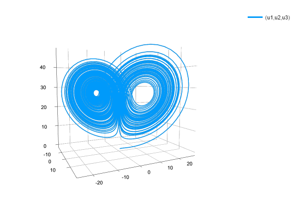
Following is an example from DifferentialEquations.jl, in which a 3-D Lorenz system is declared and solved numerically.

The Julia code of the parameterized Lorenz function looks like this:

function parameterized_lorenz!(du,u,p,t)
    du[1] = p[1]*(u[2]-u[1])
    du[2] = u[1]*(p[2]-u[3]) - u[2]
    du[3] = u[1]*u[2] - p[3]*u[3]
end

Assuming that we have already constructed the differential equations by Prolog inference and stored them in a list [E1, E2, E3], we can declare the function by jl_declare_function('parameterized_lorenz!', [:du, :u, :p, :t], [E1, E2, E3]). Following is a full example:

solve_lorenz :-
    % import useful libraries
    jl_using('DifferentialEquations'),
    jl_using('Plots'),
    
    % construct julia equations by Prolog 
    E1 = jl_expr(: (=),[jl_expr(:ref,[:du,1]),jl_expr(:call,[: (*),jl_expr(:ref,[:p,1]),jl_expr(:call,[: (-),jl_expr(:ref,[:u,2]),jl_expr(:ref,[:u,1])])])]),
    E2 = jl_expr(: (=),[jl_expr(:ref,[:du,2]),jl_expr(:call,[: (-),jl_expr(:call,[: (*),jl_expr(:ref,[:u,1]),jl_expr(:call,[: (-),jl_expr(:ref,[:p,2]),jl_expr(:ref,[:u,3])])]),jl_expr(:ref,[:u,2])])]),
    E3 = jl_expr(: (=),[jl_expr(:ref,[:du,3]),jl_expr(:call,[: (-),jl_expr(:call,[: (*),jl_expr(:ref,[:u,1]),jl_expr(:ref,[:u,2])]),jl_expr(:call,[: (*),jl_expr(:ref,[:p,3]),jl_expr(:ref,[:u,3])])])]),
    
    % declare Julia function
    jl_declare_function('parameterized_lorenz!', [:du, :u, :p, :t], [E1, E2, E3]),
    
    % set parameters
    u0 := [1.0,0.0,0.0],
    tspan := tuple([0.0,100.0]),
    p := [10.0,28.0,8/3],
    prob := 'ODEProblem'('parameterized_lorenz!',u0,tspan,p),
    
    % solve the problem and plot the result
    sol := solve(prob),
    := plot(sol, kw(vars,tuple([1,2,3])), kw(show,true)).

It will generate a nice figure like this:

Alternatively, the Function_Codes argument can be an atom referring to a Julia array of Exprs:

solve_lorenz_alt :-
    % import useful libraries
    jl_using('DifferentialEquations'),
    jl_using('Plots'),
    
    % define equations with Julia
    e := array('Any', undef, 3),
    e[1] $= du[1] = p[1]*(u[2]-u[1]),
    e[2] $= du[2] = u[1]*(p[2]-u[3]) - u[2],
    e[3] $= du[3] = u[1]*u[2] - p[3]*u[3],
    
    % declare Julia function
    jl_declare_function('parameterized_lorenz!', [:du, :u, :p, :t], e),
    ...

Arrays

Array can be initialised with function array, which is equal to Array{Type, Dim}(Init, Size) in Julia:

?- a := array('Float64', undef, 2, 2, 2).
true.

?- := @show(a[1,:,:]).
a[1, :, :] = [2.5e-322 0.0; 0.0 0.0]
true.

New arrays can also be initialised with a Prolog predicate jl_new_array/4 predicates:

% jl_new_array(Name, Type, Init, Size) works like Name = Array{Type, Dim}(Init, Size)
% in Julia, here Size is a list.
?- jl_new_array(a, 'Int', undef, [2, 2, 2]).
true.

?- := @show(a[1,:,:]).
a[1, :, :] = [34359738371 77309411345; 64424509449 140320876527618]
true.

Array initialisation also supports type unions with predicate union(Type1, Type2, ...):

?- a := array(union('Int64', 'Missing'), missing, 2, 2).
true.

?- a[1, :] := [1,2].
true.

?- := @show(a).
a = Union{Missing, Int64}[1 2; missing missing]
true.

Unifying Prolog list with multi-dimension arrays

Added a callable predicate jl_unify_arrays/0 to enable multi-dimension arrays, for example:

?- X := zeros(2,2,2).
[ERR] Cannot unify list with matrices and tensors!
false.

?- jl_unify_arrays.
true.

?- X := zeros(2,2,2).
X = [[[0.0, 0.0], [0.0, 0.0]], [[0.0, 0.0], [0.0, 0.0]]].

?- a := rand(2,2,2), 
   := display(a[1,:,:]),
   := display(a[2,:,:]),
   X := a. % unification
2×2 Matrix{Float64}:
 0.985283  0.552947
 0.545242  0.243907
2×2 Matrix{Float64}:
 0.0608626  0.056837
 0.0653907  0.354753
X = [[[0.98528283223325, 0.552946822654699], 
      [0.5452419312034834, 0.24390678160983548]], 
     [[0.060862609653857036, 0.056837009536256256], 
      [0.0653907190522306, 0.3547534277306833]]].

After enabling multi-dimension arrays, they could be unified with Prolog's nested lists:

?- jl_using('SparseArrays').
true.

?- a := sparse(zeros('Rational', 2,2)),
   a[1,1] := 1//2,
   := display(a),
   X := 'Array'(a*transpose(a)).
2×2 SparseMatrixCSC{Rational, Int64} with 1 stored entry:
 1//2   ⋅
  ⋅     ⋅
X = [[1r4, 0], [0, 0]].

Assigning a multi-dimension array with nested Prolog list via array/1 functor:

?- X = [[1,2],[3,4]],
   a := array(X), 
   := display(a).
2×2 Matrix{Int64}:
 1  2
 3  4
X = [[1, 2], [3, 4]].

Array unification problem

Jurassic seems cannot handle long array unification currently. The best workaround is to store and process large tensors in Julia.

?- X := zeros(10,10,10).
X = [[[0.0, 0.0, 0.0, 0.0, 0.0, 0.0, 0.0|...], [0.0, 0.0, 0.0, 0.0, 0.0, 0.0|...], [0.0, 0.0, 0.0, 0.0, 0.0|...], [0.0, 0.0, 0.0, 0.0|...], [0.0, 0.0, 0.0|...], [0.0, 0.0|...], [0.0|...], [...|...]|...], [[0.0, 0.0, 0.0, 0.0, 0.0, 0.0|...], [0.0, 0.0, 0.0, 0.0, 0.0|...], [0.0, 0.0, 0.0, 0.0|...], [0.0, 0.0, 0.0|...], [0.0, 0.0|...], [0.0|...], [...|...]|...], [[0.0, 0.0, 0.0, 0.0, 0.0|...], [0.0, 0.0, 0.0, 0.0|...], [0.0, 0.0, 0.0|...], [0.0, 0.0|...], [0.0|...], [...|...]|...], [[0.0, 0.0, 0.0, 0.0|...], [0.0, 0.0, 0.0|...], [0.0, 0.0|...], [0.0|...], [...|...]|...], [[0.0, 0.0, 0.0|...], [0.0, 0.0|...], [0.0|...], [...|...]|...], [[0.0, 0.0|...], [0.0|...], [...|...]|...], [[0.0|...], [...|...]|...], [[...|...]|...], [...|...]|...].

?- X := zeros(100,100,10).
X = [[[0.0, 0.0, 0.0, 0.0, 0.0, 0.0, 0.0|...], [0.0, 0.0, 0.0, 0.0, 0.0, 0.0|...], [0.0, 0.0, 0.0, 0.0, 0.0|...], [0.0, 0.0, 0.0, 0.0|...], [0.0, 0.0, 0.0|...], [0.0, 0.0|...], [0.0|...], [...|...]|...], [[0.0, 0.0, 0.0, 0.0, 0.0, 0.0|...], [0.0, 0.0, 0.0, 0.0, 0.0|...], [0.0, 0.0, 0.0, 0.0|...], [0.0, 0.0, 0.0|...], [0.0, 0.0|...], [0.0|...], [...|...]|...], [[0.0, 0.0, 0.0, 0.0, 0.0|...], [0.0, 0.0, 0.0, 0.0|...], [0.0, 0.0, 0.0|...], [0.0, 0.0|...], [0.0|...], [...|...]|...], [[0.0, 0.0, 0.0, 0.0|...], [0.0, 0.0, 0.0|...], [0.0, 0.0|...], [0.0|...], [...|...]|...], [[0.0, 0.0, 0.0|...], [0.0, 0.0|...], [0.0|...], [...|...]|...], [[0.0, 0.0|...], [0.0|...], [...|...]|...], [[0.0|...], [...|...]|...], [[...|...]|...], [...|...]|...].

?- X := zeros(100,100,100).
false.

TODO

More features to be added, e.g.:

• Multi-threading.

Compile and test code in other platform, e.g.:

• MaxOS
• Windows

Acknowledgement

The Jurassic.pl package is inspired by real (calling R from Prolog).

Another similar package is pljulia, unfortunately it is deprecated and only has limited functionalities.

Author

Wang-Zhou Dai (homepage)
School of Intelligence Science and Technology,
Nanjing University, Suzhou Campus