Hypermax is a power tool for optimizing algorithms. It builds on the powerful TPE algorithm with additional features meant to help you get to your optimal hyper parameters faster and easier. We call our algorithm Adaptive-TPE, and it is fast and accurate optimizer that trades off between explore-style and exploit-style strategies in an intelligent manner based on your results. It depends upon pretrained machine learning models that have been taught how to optimize your machine learning model as fast as possible. Read the research behind ATPE in Optimizing Optimization and Learning to Optimize, and use it for yourself by downloading Hypermax.
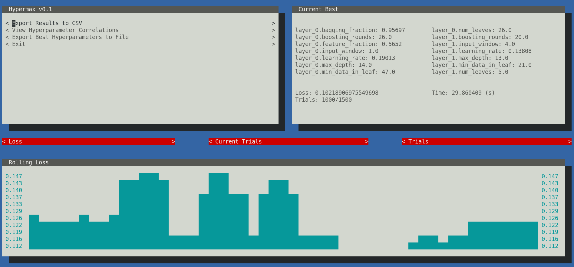
In addition, Hypermax automatically gives you a variety of charts and graphs based on your hyperparameter results. Hypermax can be restarted easily in-case of a crash. Hypermax can monitor the CPU and RAM usage of your algorithms - automatically killing your process if it takes too long to execute or uses too much RAM. Hypermax even has a UI. Hypermax makes it easier and faster to get to those high performing hyper-parameters that you crave so much.
Start optimizing today!
Install using pip:
pip3 install hypermax -gPython3 is required.
In Hypermax, you define your hyper-parameter search, including the variables, method of searching, and loss functions, using a JSON object as you configuration file.
Here is an example. Lets say you have the following file, model.py:
import sklearn.datasets
import sklearn.ensemble
import sklearn.metrics
import datetime

def trainModel(params):
    inputs, outputs = sklearn.datasets.make_hastie_10_2()

    startTime = datetime.now()

    model = sklearn.ensemble.RandomForestClassifier(n_estimators=int(params['n_estimators']))
    model.fit(inputs, outputs)
    predicted = model.predict(inputs)

    finishTime = datetime.now()

    auc = sklearn.metrics.auc(outputs, predicted)

    return {"loss": auc, "time": (finishTime - startTime).total_seconds()}
You configure your hyper parameter search space by defining a JSON-schema object with the needed values:
{
    "hyperparameters": {
        "type": "object",
        "properties": {
            "n_estimators": {
                "type": "number",
                "min": 1,
                "max": 1000,
                "scaling": "logarithmic"
            }
        }
    }
}
Next, define how you want to execute your optimization function:
{
    "function": {
        "type": "python_function",
        "module": "model.py",
        "name": "trainModel",
        "parallel": 1
    }
}
Next, you need to define your hyper parameter search:
{
    "search": {
        "method": "atpe",
        "iterations": 1000
    }
}
Next, setup where you wants results stored and if you want graphs generated:
{
    "results": {
        "directory": "results",
        "graphs": true
    }
}
Lastly, you need to provide indication if you want to use the UI:
{
    "ui": {
        "enabled": true
    }
}
NOTE: At the moment the console UI is not supported in Windows environments, so you will need to specify false in
the enabled property. We use the urwid.raw_display module which relies on fcntl. For more information, see here.
Pulling it all together, you create a file like this search.json, defining your hyper-parameter search:
{
    "hyperparameters": {
        "type": "object",
        "properties": {
            "n_estimators": {
                "type": "number",
                "min": 1,
                "max": 1000,
                "scaling": "logarithmic"
            }
        }
    },
    "function": {
        "type": "python_function",
        "module": "model",
        "name": "trainModel",
        "parallel": 1
    },
    "search": {
        "method": "atpe",
        "iterations": 1000
    },
    "results": {
        "directory": "results",
        "graphs": true
    },
    "ui": {
        "enabled": true
    }
}
And now you can run your hyper-parameter search
$ hypermax search.jsonHypermax will automatically begin searching your hyperparameter space. If your computer dies and you need to restart your hyperparameter search, its as easy as providing it the existing results directory as a second parameter. Hypermax will automatically pick up where it left off.
$ hypermax search.json results_0/Hypermax supports 4 different optimization algorithms:
- "random" - Does a fully random search
- "tpe" - The classic TPE algorithm, with its default configuration
- "atpe" - Our Adaptive-TPE algorithm, a good general purpose optimizer
- "abh" - Adaptive Bayesian Hyperband - this is an optimizer that its able to learn from partially trained algorithms in order to optimizer your fully trained algorithm
The first three optimizers - random, tpe, and atpe, can all be used with no configuration.
The only optimizer in our toolkit that requires additional configuration is the Adaptive Bayesian Hyperband algorithm.
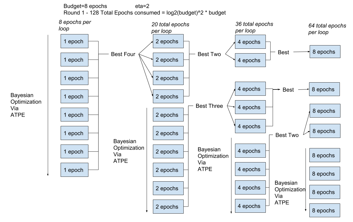
ABH works by training your network with different amounts of resources. Your "Resource" can be any parameter that significantly effects the execution time of your model. Typically, training-time, size of dataset, or # of epochs are used as the resource. The amount of resource is referred to as the "budget" of a particular execution.
By using partially trained networks, ABH is able to explore more widely over more combinations of hyperparameters, and then triage the knowledge it gains up to the fully trained model. It does this by using a tournament of sorts, promoting the best performing parameters on smaller budget runs to be trained at larger budgets. See the following chart as an example:
There are many ways you could configure such a system. Hyperband is just a mathematically and theoretically sound way of choosing how many brackets to run and with what budgets. ABH is a method that combines Hyperband with ATPE, in the same way that BOHB combines Hyperband with conventional TPE.
ABH requires you to select three additional parameters:
- min_budget - Sets the minimum amount of resource that must be allocated to a single run
- max_budget - Sets the maximum amount of resource that can be allocated to a single run
- eta - Defines how much the budget is reduced for each bracket. The theoretically optimum value is technically E or 2.71, but values of 3 or 4 are more typical and work fine in practice.
You define these parameters like so:
{
  "search": {
      "method": "abh",
      "iterations": 1000,
      "min_budget": 1,
      "max_budget": 30,
      "eta": 3
  }
}
This configuration will result in Hyperband testing 4 different brackets: 30 epochs, 10 epochs, 3.333 epochs (rounded down), and 1.1111 epochs (rounded down)
The budget for each run is provided as a hyperparameter to your function, along side your other hyperparameters. The budget will be given as the "$budget" key in the Python dictionary that is passed to your model function.
Tips:
- ABH only works well when the parameters for a run with a small budget correlates strongly with the parameters for a run with a high budget.
- Try to eliminate any parameters whose behaviour and effectiveness might change depending on the budget. E.g. a parameter for % of budget in mode 1, % of budget in mode 2 will not work well with ABH.
- Don't test too wide of a range of budgets. As a general rule of thumb, never set min_budget lower then max_budget/eta^4
- Never test a min_budget thats so low that your model doesn't train at all. The minimum is there for a reason
- If you find that ABH is getting stuck in a local minima, choosing parameters that work well on few epochs but work poorly on many epochs, your better off using vanilla ATPE and just training networks fully on each run.
Hypermax automatically generates a wide variety of different types of results for you to analyze.
The hyperparameter correlations can be viewed from within the user-interface or in "correlations.csv" within your results directory. The correlations can help you tell which hyper-parameter combinations are moving the needle the most. Remember that a large value either in the negative or positive indicates a strong correlation between those two hyper-parameters. Values close to 0 indicate that there is little correlation between those hyper-parameters. The diagonal access will give you the single-parameter correlations.
It should also be noted that these numbers get rescaled to fall roughly between -10 and +10 (preserving the original sign), and thus are not the mathematically defined covariances. This is done to make it easier to see the important relationships.
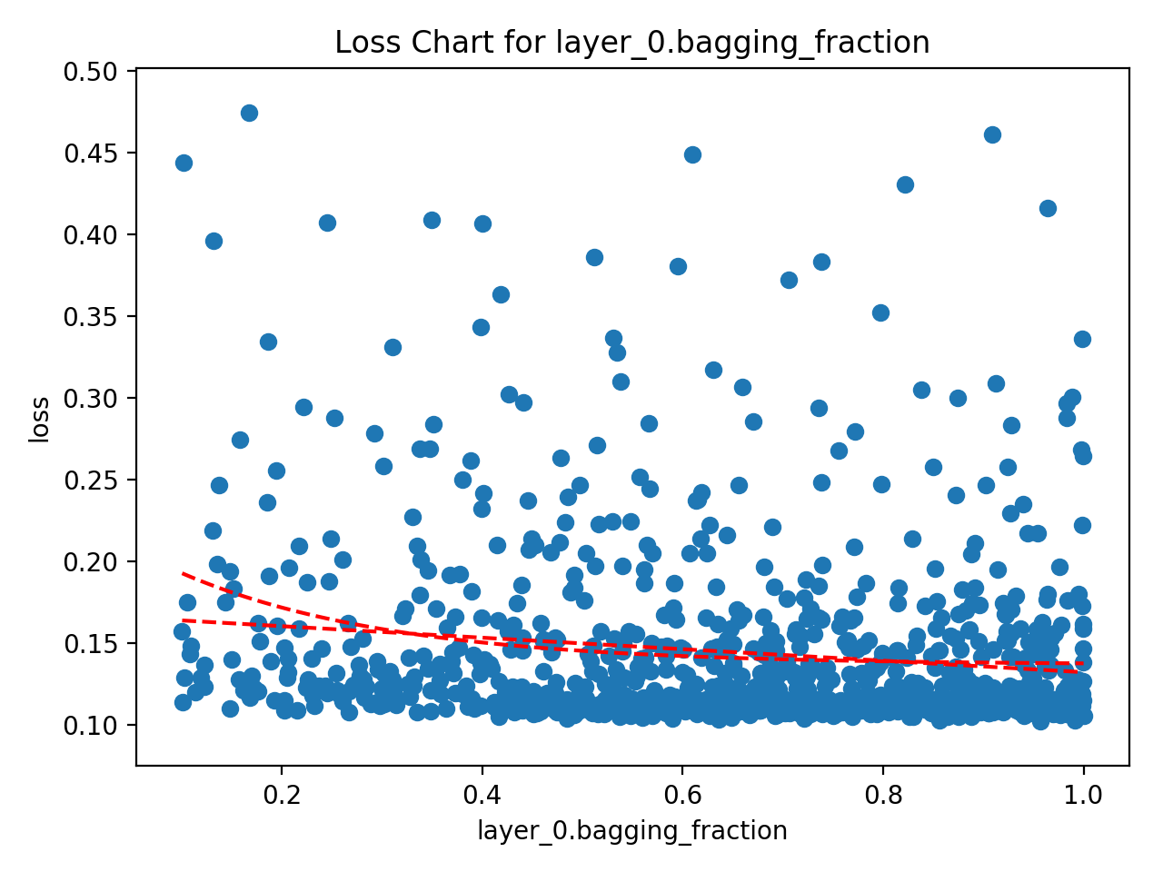
The single parameter loss charts create a Scatter diagram between the parameter and the loss. These are the most useful charts and are usually the go-to for attempting to interpret the results. Hypermax is going to generate several different versions of this chart. The original version will have every tested value. The "bucketed" version will attempt to combine hyper-parameter values into "buckets" and give you the minimum value for each bucket - useful for continuous valued hyper-parameters that you have a lot of results for. The "top_10_percent" version is just showing you the scatter for only the top-10% of results - useful when you want to home in on those top-performing values.
You will also get a version of this chart for the time that your model takes to execute. This can be useful if trading off between accuracy and time taken is important to you.
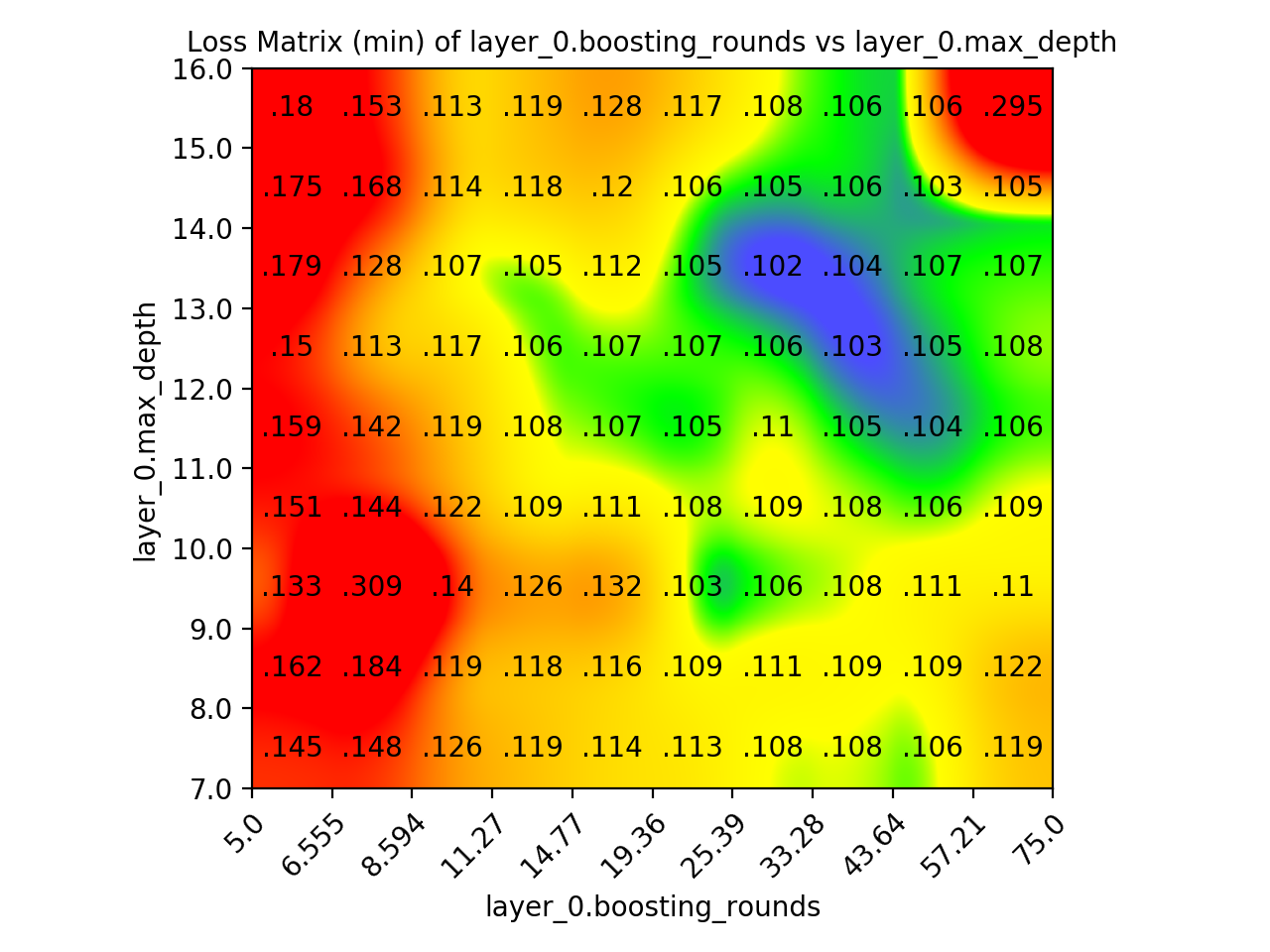
The two parameter loss matrixes are a color-coded diagram that helps you to determine the optimal value between two hyper-parameters.
The graph is color coded in the following way:
Red: 90th percentile of squares
Yellow: 40th percentile of squares
Green: 20th percentile of squares
Blue: 5th percentile of squares
We use quadric interpolation which both gives nice smooth rounded corners but does not excessively blur key areas. Thee chart is generated by dividing your hyperparameter values into 10 buckets each, resulting in a 10x10 grid of squares. We compute a value for each square in two ways:
One version of the graph computes the value for each square by taking the Min of all values in that grid square. This is usually the most useful chart. The other version computes the value by taking the Mean. This second version can be susceptible to outlier results, but can show interesting patterns sometimes.
You also get versions of this graph done which only use the top 10% of your results, helping you to further focus in on the top performing area of your hyper parameter space. In addition, you get a version of this matrix done for the execution time of your model - in caes that is important.
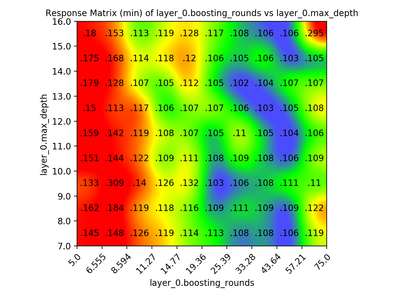
The response matrixes are very similar to the Loss matrices. In fact - it displays all of the same data. They are just color-coded differently to highlight different things. The Loss matrix defines its colors based on global statistics. The Response Matrix defines its colors based only one the values within each row. This often highlights important patterns - such as that the optimal value for one hyperparameter is always the same, regardless of the other hyper parameter (like this chart below, where optimal boosting_rounds appears to be around 40, no matter what the max_depth is.)
The graph is color coded in the following way:
Red: 90th percentile of row
Yellow: 60th percentile of row
Green: 30th percentile of row
Blue: 10th percentile of row
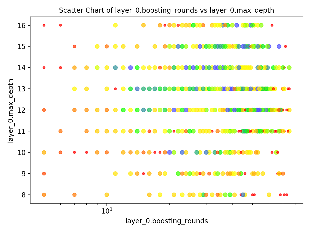
The two parameter scatters go along-side the two-parameter loss matrices. If you are concerned that the Loss Matrixes may be trying to extrapolate too much from very few data-points, you can check the scatter in order to check if you actually have a decent sample of results that fall within that area.
The color coding is the same as it is for the Loss Matrix, but percentiles are calculated over all results and not over the 10x10 grid of squares.
Red: 90th percentile of values
Yellow: 40th percentile of values
Green: 20th percentile of values
Blue: 5th percentile of values
The size of the markers will also vary - larger and bluer is more accurate. Smaller and redder is less accurate.
For all of the above mentioned charts, you will automatically get CSV files containing all of the raw data used to generate that chart.
You define your hyper-parameter space within the "hyperparameters" section of the configuration file. The format is reminiscent of JSON-schema, however, only a limited set of options are supported.
Most of the hyper-parameters that you are going to be tuning are expected to be numbers. The configuration of the number hyper-parameter looks like so:
{
    "parameter_name": {
        "type": "number",
        "mode": "uniform",
        "scaling": "logarithmic",
        "min": 1,
        "max": 1000,
        "rounding": 1
    }
}
There are 3 required parameters - type, min and max. Type should be set to 'number', and the min and max should represent the minimum and maximum values of your range.
There are also three optional parameters. mode can be either uniform or normal (defaults to uniform). The scaling parameter can be either linear
or logarithmic (default to linear). And you can additionally set rounding if you want values to be rounded to some fixed interval. A rounding set to 1
will make your parameter an integer.
When you have several different possible values that are categorically distinct, you can use an enumeration to specify the possible options:
{
    "activation_function": {
        "type": "string",
        "enum": ["relu", "elu", "tanh", "sigmoid", "swish", "prelu", "selu"]
    }
}Your hyper-parameter space can contain JSON objects which contain other hyper parameters. In fact, the bottom layer must be made as an object. Simply
set the type to object and provide it a properties field.
{
    "parameter_object": {
        "type": "object",
        "properties": {
            "parameter_name": {
                "type": "number",
                "mode": "uniform",
                "scaling": "logarithmic",
                "min": 1,
                "max": 1000,
                "rounding": 1
            }
        }
    }
}The true power of the TPE algorithm comes from its ability to optimize categorical hyper-parameters, including ones which make other hyper-parameters
available. To do this, you can provide either a oneOf or anyOf field. Note that "oneOf" and "anyOf" behave exactly the same - we allow
both in order to match JSON-Schema specifications.
{
    "choice_parameter": {
        "anyOf": [
            {
                "type": "object",
                "properties": {
                    "parameter_name": {
                        "type": "number",
                        "min": 1,
                        "max": 1000
                    }
                }
            },
            {
                "type": "object",
                "properties": {
                    "other_parameter_name": {
                        "type": "number",
                        "min": 1,
                        "max": 1000
                    }
                }
            }
        ]
    }
}
Hypermax will add in an additional "parameter_name.$index" field into the parameters it sends to your algorithm, so that you can tell which side of the branch you are on.
Important! When using oneOf or anyOf, each of the options MUST be "object" type hyperparameters, as shown above.
When using decision points, you may find it convenient to add in a constant value to tell you which side of the branch you are on.
This is easy using a "constant" parameter. You can have the same parameter name on both sides of the branch.
This allows you to, for example, test two different neural network optimizers, and the various learning rates attached to each, without having to worry that the algorithm is going to learn an "average" learning rate that works for both optimizers. Both sides of the branch will be kept separate during optimization, even though they share the same parameter names.
Constant parameters are ignored for optimization purposes, but are still passed into your function, making them mostly useful when you want to lock in a parameter without changing your code, or when using decision points like so:
{
    "optimizer": {
        "oneOf": [
            {
                "type": "object",
                "properties": {
                    "optimizerName": {
                        "type": "string",
                        "constant": "adam"

                    },
                    "learningRate": {
                        "type": "number",
                        "min": 1e-5,
                        "max": 1e-3
                    }
                }
            },
            {
                "type": "object",
                "properties": {
                    "optimizerName": {
                        "type": "string",
                        "constant": "sgd"

                    },
                    "learningRate": {
                        "type": "number",
                        "min": 1e-5,
                        "max": 1e-3
                    }
                }
            }
        ]
    }
}There are several different ways of executing your model.
The most straight forward way to execute your model is by defining a Python function. To do this, simply provide the name of the module and the name of the function in the "module" and "name" functions, like so:
{
    "function": {
        "type": "python_function",
        "module": "model",
        "name": "trainModel"
    }
}
Remember that you do not include the extension of the name of your module, there is no ".py" on it. The module is referenced using Pythons standard system. This means that you can directly reference any files in the current working directory simply by their file-name. Alternatively, you can reference a system-package or a Python package that is setup elsewhere. As long as this works:
    $ python3

    Python 3.6.5 (default, Mar 29 2018, 18:20:46)
    [GCC 8.0.1 20180317 (Red Hat 8.0.1-0.19)] on linux
    Type "help", "copyright", "credits" or "license" for more information.
    >>> import module_name
    >>> module.foobar()
Then this will to:
{
    "function": {
        "type": "python_function",
        "module": "module_name",
        "name": "foobar"
    }
}The results can be provided in one of two formats. The simplest is to just return the loss directly as a single floating point value from your cost function, or print it to standard output in your executable. For example:
def trainModel(parameters):
    # Do some fancy stuff
    loss = 1.0
    return loss
or as an executable:
#!/usr/bin/python3

# Do some fany stuff
loss = 1.0
print(loss)
If you are using multiple losses though, you will have to return each of them as part of a JSON object. For example:
def trainModel(parameters):
    # Do some fancy stuff
    accuracy = 0.9
    stddev = 0.1
    return {"accuracy": accuracy, "stddev": stddev}
or as an executable:
#!/usr/bin/python3

import json

# Do some fancy stuff
accuracy = 0.9
stddev = 0.1
print(json.dumps({"accuracy": accuracy, "stddev": stddev}))
If you want to store additional metadata with your model, you can. Any fields that are unrecognized for any other purpose will be automatically considered as metadata.
def trainModel(parameters):
    # Do some fancy stuff
    loss = 1.0
    additional_statistic = 42.0
    return {"loss": loss, "additional_statistic": additional_statistic}
The time your model takes is automatically measured by Hypermax (time can be used for punishing your model for taking too long, see Losses section).
However, you may only care about the execution / run-time of your model, and not about the training time. In these cases, you can return time as
an additional variable.
def trainModel(parameters):
    # Do some fancy stuff
    model = Model()
    model.train()
    start = datetime.now()
    loss = model.test()
    end = datetime.now()
    return {"loss": loss, "time": (end-start).total_seconds()}
It should be noted that this time is not the same time used for auto_kill purposes. This is the time that will be showed in the UI and considered for optimization
purposes.
Sometimes, your models may be behaving very poorly in certain parts of your hyper-parameter space. It is thus possible, and indeed recommended, to set add limits on how long your model can be running for and how much RAM it can use. This prevents your optimization routine from getting hung due to a model that takes too long to train, or crashing entirely because it uses too much RAM.
To do this, simply add in a auto_kill_max_time, auto_kill_max_ram, or auto_kill_max_system_ram option, and set a
a kill_loss variable to indicate what the loss should be for models which are killed.
auto_kill_max_time is specified in seconds. auto_kill_max_ram and auto_kill_max_system_ram are both specified in
megabytes, the kind which are based by 1024 (not 1000).
auto_kill_max_ram only measures the RAM of the model process. However, if your cost-function has other various
sub-processes which take up RAM, these will not be counted. Therefore, you can use auto_kill_max_system_ram in
these cases to prevent total system RAM usage from creeping too high (the assumption being your model is what is
taking up the systems RAM). You are able to provide both at the same time (if you want to).
auto_kill_loss is just a floating point indicating the total loss that should be given to the optimizer when the model
is killed. This helps teach the optimizer to avoid hyper-parameters which lead to models being killed.
{
    "function": {
        "type": "python_function",
        "module": "model",
        "name": "trainModel",
        "auto_kill_max_time": 120.0,
        "auto_kill_max_ram": 512,
        "auto_kill_max_system_ram": 3800,
        "auto_kill_loss": 1.0
    }
}PLEASE NOTE THIS SECTION IS DESCRIBING FUTURE FUNCTIONALITY AND IS NOT YET SUPPORTED. PLEASE IGNORE THIS SECTION.
We support several different types of cost functions.
You can include the time your model takes to train as one of your loss functions as well. This makes it convenient to teach the algorithm to avoid bad hyper parameters which lead to long training times. Many algorithms have poor combinations of parameters which can lead to long execution time with no improvement in performance.
If the algorithm takes less then the target_time, then no penalty is incurred. As the time taken goes between
target_time and max_time, the penalty is introduced quadratically. At max_time, the penalty is exactly
penalty_at_max.
This usually results in the algorithm choosing a value between target_time and max_time, but closer
to target_time. For example, with the following:
{
    "metrics": {
        "time": {
            "type": "time",
            "target_time": 5,
            "max_time": 10,
            "penalty_at_max": 0.1
        }
    }
}
If the algorithm takes 5.0 seconds, no penalty is introduced. At 6.0 seconds, the penalty is:
= ((6 - 5) ^ 2 / (10 - 5)^2)*0.1
= 0.0025
At 9 seconds, the penalty is:
= ((9 - 5) ^ 2 / (10 - 5) ^ 2)*0.1
= 0.064
At 10 seconds, the penalty is:
= ((10 - 5) ^ 2 / (10 - 5) ^ 2)*0.1
= 0.1
Longer times will have even larger penalties.
See here:
Feel free to contribute! Reach out to Brad at [email protected] or here on Github. We welcome additional contributors.
This is the grand-todo list and was created on August 4, 2018. Some items may have been completed.
- Results
- Able to configure save-location.
- Automatic uploading of results to Google Drive
- Model Execution
- Autokill models that take too much GPU RAM
- Autokill models that take too much Disk / Network (not sure about this one)
- Fix bug related to using too many file handlers.
- Execute model as an executable
- Execute model remotely, through ssh
- Execute model by sending a message through message-buffer like RabbitMQ or Kafka (receive results same way)
- Rsync a folder prior to remote execution
- Can attach additional arbitrary metadata to your model results
- Able to have "speed-tests" on models, where your hyper-parameters are tested on a reduced dataset in order to measure the speed. Useful to eliminate bad hyper-parameters without executing the full model.
- Similarly, able to run "memory tests" on models, ensuring your hyper-parameters don't lead to excessive ram usage
- Able to automatically run additional cross-folds on your best-models, to ensure they aren't statistical flukes
- Hyper-parameters with rounding set to 1 should be automatically converted to integer
- Configuration:
- JSON-schema for the configuration files
- validation of json-schemas
- Ability to accept yaml as well as JSON
- Able to have fixed values inside of the hyper-parameter schemas.
- Able to have "unbounded" hyperparameters (only when using iterative optimization, since TPE doesn't inherently do this)
- Ability to have hyper-parameters within arrays, such as a list of layers
- Reliability:
- Hypermax saves results / reloads from where it left off by default
- Try to lock in package versions related to Hyperopt so people don't have problems on installation
- Need a better way of handling exceptions that happen in UI code
- Execution threads should only communicate through queues, eliminate shared variables (and put locks in the ones we can't eliminate)
- Control random seed and ensure that runs are reproducible
- General User Interface:
- Change User-Interface code to use proper organized classes and not ad-hoc style like it is currently
- View recently trained models
- Able to view Training Loss VS. Testing Loss on UI
- View models which had errors
- Fix UI issues related to data-tables (such as in hyperparameter correlations)
- Able to adjust min,max,smoothing, and domain of the loss chart
- Predict model execution time based on hyper-parameters and prior data
- Progress-bar on model training
- Can change the file-name when exporting the hyper-parameter correlations
- Can instantly open files which are exported, using xdg-open & equivalents
- Widget which allows easily viewing/scrolling a large block of text.
- View the raw hyper-parameter search configuration, as JSON
- Exporting the hyper-parameters should save them in the exact format they are fed into the model, not in a flattened structure
- View the hyper-parameter space while model is running
- Can view arbitrary metadata that was attached to models
- Make the UI responsive to different console sizes (like a grid system)
- Fix the bug where the UI doesn't automatically resize when terminal resizes
- Access the UI through a web-browser
- Password-protection on web-browser UI
- Able to monitor the RAM (and GPU RAM) usage of currently executing models
- Able to monitor the disk usage of currently executing models
- Able to monitor the network usage of currently executing models
- Able to monitor general system stats, such as CPU, network, disk, and ram
- Losses:
- Able to have multiple weighted loss functions
- Automatically pass loss-function through math-function based on min,max,target to add in asymptotes at target values
- Write documentation related to how your cost-function is manipulated to improve results
- Convenient way to add Time as an additional loss on your model
- Time computed automatically, but can be overridden if provided in results
- Can view all the losses for a given model in the UI, not just final loss
- Convenient way to add in peak or median RAM (and GPU RAM) as an additional loss on your model
- Convenient way to add in disk / network usage as a additional loss on your model
- Tools for Hyperparameter Tuning:
- Improve feature-vector design for hyper-parameter correlations
- Edit / change the hyper-parameter space while the model is running
- Estimate the cardinality of the search-space
- Estimate number of runs per parameter (or something like this)
- Ability to fit a hyper-model and do a simulated extension of your hyper-parameter search, trying to predict if there are better values that you haven't searched
- Ability to use the hyper-model to hold certain hyper-parameters constant, and determine the optimal values for remaining hyper-parameters
- Staged tuning - able to have multiple tuning "stages", which tune only certain hyper-parameters at a time or with different configurations
- Can have a 'default' value for each of the hyperparameters, e.g. your current best model.
- Incremental tuning - basically only tunes a handful of hyper-parameters at a time. Can be random or specified
- Ability to change the hyper parameters for TPE
- Research some automatic way to guess good TPE hyper-parameters
- Integrate Bayesian hyper-parameter optimization as an alternative to TPE
- Integrate grid-search as an alternative to TPE
- Integrate genetic-algo as an alternative to TPE
- Command-line interface
- Execute model without CUI
- Sample next hyper-parameters to test
- Export all of the existing types of result-analysis (correlations, hotspot-grids, param vs loss, etc..)
- Launch web browser UI (without CUI)
- Write a template configuration file to the current directory
- Library interface:
- Able to activate hypermax by calling a library function
- Able to provide our cost-function directly as a python function, rather then just as a JSON description
- Testing
- Write unit tests for hyper-parameter configuration
- Write unit tests for model execution
- Write unit tests for loss functions
- Write unit tests for the optimizer
- Write unit tests for the results generation
- Write unit tests related to reliability (starting / stopping models)
- Write unit tests for command line interface
- Write unit tests for web-UI module (just ensure it loads)
- Write UI tests for the CUI
- Write end-to-end optimization tests for a few different real datasets / algos
- Template hyperparameter spaces:
- Create a template hyper-parameter search for lightgbm
- Create a template hyper-parameter search for xgbboost
- Create template hyper-parameter searches for various scikit-learn estimators
- Ability to reference template hyper-parameter searches in your own JSON schemas ($ref)
- Release / Launch:
- Test hypermax in following environments, and fix any issues with installation configuration
- Fresh virtual environment
- Fresh fedora installation
- Fresh ubuntu installation
- macOS
- Write all the documentation for the README file for Hypermax
- Create Github wiki, duplicate README documentation in Github Wiki
- Create Hypermax web-page as sub-domain of Electric Brain, duplicate information from README
- Write a blog post discussing hypermax and hyper-optimization in general
- Create optimization examples for:
- Python
- Java
- NodeJS
- Ruby
- R
- Create system packages for:
- Fedora / Redhat / CentOS
- Debian / Ubuntu
- macOS
- Windows
- Test hypermax in following environments, and fix any issues with installation configuration
