New functions

Two executable scripts were added in the src/explore_erdbeermet package.

• rmet.py
• equations_extended.py

Required packages

Currently explore_erdbeermet relies on some external python packages:

pip install pyvis
pip install pathlib
pip intall numpy
pip intall contextlib
pip install sympy
pip install texttable
pip install itertools

should do the trick. Furthermore, you should install the "canonical" erdbeermet first, and replace its installation in site_packages by the erdbeermet version included in this repository.

Additionally, you need to change Line 167 in src/explore_erdbeermet/rmet.py to point to your own splitstree installation if you desire to explore Scenarios visualized as SplitsTree. Just remove Line 167/168 if you do not want to currently use this function.

rmet.py

Is intended to allow for an interactive exploration of the algorithm erdbeermet utilizes. It loads a scenario (custom format) from a file and applies the erdbeermet recognition algorithm. A network visualization, the usual .pdf output from erdbeermet, and a splitstree image is generated.

Example vis (of star1 example):

Splitstree:

Network:

Usage:

Execute from base directory:

python src/explore_erdbeermet/rmet.py <SCENARIO-FILE> <NEXUS-OUTPUT(SplitsTree)> <PNG-OUTPUT(SplitsTree)> <SIMFILE-OUTPUT>

This simple example reads the star scenario that is provided in the examples folder and writes all output to the output folder:

python src/explore_erdbeermet/rmet.py examples/explore_erdbeermet/star1 output/star.nex output/star.png output/simfile_star

Follow the instructions in the command prompt to explore the scenario you have loaded.

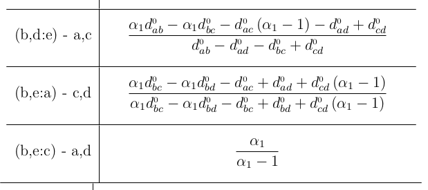
At each step, rmet.py outputs a list of possible Reverse-R-step candidates which are sorted by the sum of invalid alphas (over all witness combinations). All possible candidates are outputted and you find the "valid-alpha-candidates" at the bottom of the list. Each candidate is represented as:

(x,y:z) - [sum_invalid_alphas] || alpha_1:#support ... alpha_n:#support

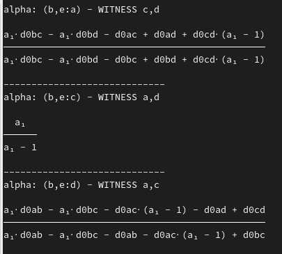
When you scroll up further, the steps in calculating the alphas for each candidate is outputted. Generally, four options are availiable:

• press R - Perform reverse R-step (permanent for current run; scenario files are not altered)
• press C - to compare 2 candidates by (temporarily) hybridizing/spike some valid candidates and observe the alphas these new witnesses yield. Each spike/hybridization is presented in a separate output section.
• press S - to examine a single candidate rev-R-step. New alphas for hybridization and the corresponding calculations are outputted as well as the deltas for this R-step (across different witnesses). Output is similar to "C".
• press G - to examine a group of candidates, i.e. 1,2:3 ; 1,2:4 ; 1,2:0 to apply the procedure of reverse-alpha-checking to these pairs.

Most options require further input from the user, i.e. to choose candidates to examine. Input prompts should be self explainatory.

You may be required to change the SplitsTree4 path in rmet.py to point to your SplitsTree4 installation to produce the SplitsTree images (LINE 167 in src/explore_erdbeermet/rmet.py).

equations_extended.py

Symbolically computes an R matrix from a given scenario file. Every distance beyond the first four leaves is computed as a term of the distances of the root leaves (first four). The distance d_0xy correspond to distances of the first four leaves. The variables del0_e, del_1, etc. correspond to deltas at the corresponding R-Steps (index start at R-Step 5; hence del0_e is the delta applied to e at the fifth R-Step). This concept carries over to alphas, e.g. a0, a1, etc.. A LaTeX .pdf as well as a console output containing the alpha-formulas for reverse R steps with respect to different witnesses is presented.

Example Output:

LaTeX:

Console

Usage:

Execute script from any directory and pass the scenario file as the first argument, and the output .tex file as the second argument.

python equations_extended.py <PATH-TO-SCEN-FILE> <OUT.TEX>

A simple call from the base directory with the star example would be:

python src/explore_erdbeermet/equations_extended.py examples/explore_erdbeermet/star1 output/star.tex

Altered Format of Scenario files:

a,b,c,d,e,f             # first row contains symbols for elements
a                       # second row contains starting leaf
a,a,b;1,0,0,1           # all following rows describe R-Steps
a,b,c;0.5,0,0,1         # i.e. x,y,z;alpha,deltax,deltay,deltaz
a,b,d;0.5,0,0,1
b,c,e;0.5,0,0,1
a,e,f;0.5,0,0,1         # empty lines at the end lead to termintation

##basic_eq.py

Is supposed to be imported (from basic_eq import *) to manually manipulate or calculate alphas. It is loaded with a baseline scenario on 5 leaves. x,y,u and v are the origin leaves and z is added as (x,y:z). You can calculate alpha by invoking calc_a(). See the script for the parameters. Symbolic distance variables can be accessed, e.g., as xy0, uv0, uz1, xz1, etc. . The distance variables are "lexiographic" - ux0 can be accessed, xu0 is not defined.

---

Erdbeermet

A Python library for generating, visualizing, manipulating and recognizing type R (pseudo)metrics (German: Erzeugung, Darstellung, Bearbeitung und Erkennung von R-(Pseudo)Metriken).

Installation

Download or clone the repo, go to the root folder of package and install it using the command:

python setup.py install

Dependencies

The package requires Python 3.7 or higher.

• Numpy
• Scipy
• Matplotlib

Usage and description

Simulation

Background

R matrices are defined as distance matrices that can be obtained by repeated merge and branching events (see Prohaska et al. 2017 and the simulation steps below), the so-called "R-steps".

The construction of any R matrix D starts with a single item (0 in the simulation). The second item (1) is always created by a pure branching event. The construction then continues with a series of merge and branching events until N items have been created.

In the simulation, every such iteration is executed as follows (the distances are always updated symmetrically, i.e., such that D[i, j] = D[j, i]):

• with probability branching_prob, execute a pure branching event
  • choose x randomly among the existing items
  • create a new item z such that D[u,z]=D[x,z] for all previously created items u (in particular D[x,z]=0.0)
• otherwise, execute a merge event
  • choose parents x and y randomly (if circular=True, they must be neighbors in a circular order that is maintained simultaneously to the simulation)
  • choose alpha from a uniform distribution on the interval (0, 1)
  • create a new item z
    • set D[x, z] = (1 - alpha) * D[x, y] and D[y, z] = alpha * D[x, y]
    • set D[u, z] = alpha * D[x, u] + (1 - alpha) * D[y, u] for all other previously created item u
    • if circular=True, insert z between x and y in the circular order
• for each item p created so far (including z), draw a distance increment delta[p] (here from an exponential distribution with rate parameter 1.0), if clocklike=True draw a common distance increment for all items
• set D[p, q] = D[p, q] + delta[p] + delta[q] for all pairs p, q of items

A simulation therefore can be stored as a history (see below), i.e., a list of the R-steps, each comprising a merge event of x and y that creates z with a parameter alpha (if alpha is 0 or 1, we have a pure branching event), and additionally a list of distance increments ("deltas") for the currently existing items.

A history written to file has one line per R-step of the form (x, y: z) alpha; [deltas].

Example file: (Click to expand)

(0, 0: 1) 1.0; [0.26,0.11]
(1, 0: 2) 0.27; [0.004,0.18,0.2]
(1, 2: 3) 0.61; [0.49,0.08,0.37,0.17]
(0, 3: 4) 0.82; [0.21,0.06,0.03,0.42,0.02]
(1, 4: 5) 0.81; [0.02,0.004,0.08,0.11,0.01,0.04]

The class Scenario

The module erdbeermet.simulation contains functions for simulating R matrices, writing simulated scenarios to file, and reloading them. The class Scenario acts as a wrapper for histories of merge and branching events and the corresponding R matrix.

The class has the following attributes: (Click to expand)

Attribute	Type	Description
N	int	the number of items that were simulated
history	list of tuples	the history of merge and branching events
circular	bool	indicates whether the scenario has a circular type R matrix
D	NxN numpy array	the distance matrix

and the following functions: (Click to expand)

Function	Parameter/return type	Description
distances()	returns NxN numpy array	getter for the distance matrix
get_history()	returns list of tuples	getter for the event history
get_circular_order()	returns list of ints	list representing the circular order (cut between item 0 and its predecessor); or False if the scenario is not circular
write_history(filename)	parameter of type str	write the event history into a file
print_history()		print the event history

Generation of Scenarios

Instances of Scenario can be generated using the function simulate() in the module erdbeermet.simulation.

Parameters of this function (Click to expand)

Parameter (with default values)	Type	Description
N	int	number of items to be generated
branching_prob=0.0	float	probability that an event is a pure branching event; the default is 0.0, i.e., pure branching events are disabled
circular=False	bool	if set to True, the resulting distance matrix is guaranteed to be a circular type R matrix (only "neighbors" can be involves in merge events)
clocklike=False	bool	if set to True, the distance increment is equal for all items within each iteration (comprising a merge or branching event and the distance increments) and only varies between iteration; the default is False, in which case the increments are also drawn independently for the items within an iteration

Simulated scenarios can be saved to a file (in form of their event history) using their function write_history(filename).

from erdbeermet.simulation import simulate, load

# simulate a scenario with six items
scenario = simulate(6, branching_prob=0.3, circular=True, clocklike=False)

# print the individual R-steps
scenario.print_history()

# write history to file
scenario.write_history('path/to/history.txt')

# reload history to file
scenario_reloaded = load('path/to/history.txt')

Alternatively, the function load(filename, stop_after=False) returns an instance of Scenario after reading an event history from an earlier simulated scenario from a file. The parameter stop_after can be set to an int x>0 to only include the R-steps until the x'th item is created, i.e., x-1 R-steps are executed.

Recognition

Background

Recognition of R matrices works by identifying a candidate for the last R-step (x, y: z) alpha, removing z from the distance matrix, and updating the distances according to specific rules. This process is repeated until certain conditions are no longer satisfied (in which case the reconstruction path is not a valid reconstruction of the history) or until only 4 items remain. A distance matrix on 4 items can be recognized as an R matrix using a specific formula.

A problem arises as there are often multiple candidates for the last R-step. Multiple cases can occur for a specific candidate:

• it is the true last R-step
• it is one of the true last R-steps (that happened in different branches and did not take part in any merging event later)
• it is not an R-step that occurred in the "true" history but it admits the reconstruction of an alternative history that produces the same R matrix
• it is not an R-step that occurred in the "true" history and we will eventually hit a "dead end" if we choose this candidate no matter which candidate decisions we make later

The last point is critical since it implies that we have to try all candidates (unless we find more conditions to rule out candidates or a completely different algorithm). Since this is true for every iteration, there is a possibly exponential number of reconstruction paths that have to be checked. If a valid R matrix is given as input, at least one of these paths will return a successful reconstruction of a history that explains it.

The module erdbeermet.recognition currently follows this approach, i.e., it tries all possible candidates. The overall recognition process can therefore be represented by a tree with the root representing the full input distance matrix and every vertex having one children per candidate R-step (x, y: z) alpha. Moreover, every such child is associated with the distance matrix obtained by removing the line and column corresponding to z and updating the remaining distances accordingly. A vertex is a leaf when it has no valid candidate R-steps or none of them produces an updated distance matrix that still satisfies certain necessary conditions of R matrices (pseudometric, ...). Also, vertices corresponding to 4x4 matrices are always leaves as, for them, it can be decided immediately whether or not they are R matrices.

Recognition trees

The function recognize(D) in the module erdbeermet.recognition takes a distance matrix D as input and returns the recognition tree as described in the previous section (instance of type Tree with attribute root of type TreeNode).

The tree nodes have the following attributes: (Click to expand)

Attribute	Type	Description
parent	TreeNode	the parent node (None for the root)
children	list of TreeNodes	child node (empty for the leaves)
n	int	the number of remaining items
V	list of ints	the list of remaining items
D	nxn numpy array	the distance matrix
R_step	tuple	the last R-steps that was identified and used to obtain D from the parents n+1xn+1 matrix (order x, y, z, alpha); equals None for the root
valid_ways	int	total number of recognition paths leading to a success in the subtree below this node
info	str	info string why the recognition failed after the application of the R-step (if this is the case)

The input distance matrix was an R matrix if recognition_tree.root.valid_ways > 0 for the recognition_tree returned by the function recognize(D).

This function has an optional parameter first_candidate_only (default False) which, when set to True, results in the algorithm only considering the first valid candidate R-step (that also produces a pseudometric and non-negative deltas) in every iteration. As a consequence, the algorithm is guaranteed to finish in polynomial time. However, it may encounter a "dead end" even though the input was an R matrix.

The function also has an optional parameter print_info (default False). When it is set to True, information on the ongoing recognition is printed to the console.

There are several ways to output/analyze the result of a recognition, i.e., the recognition tree:

from erdbeermet.simulation import simulate
from erdbeermet.recognition import recognize

# simulate scenario (alternatively load from file or create a custom distance matrix) and recognize
scenario = simulate(6)
recognition_tree = recognize(scenario.D, print_info=True)

# write the recognition steps into a file
recognition_tree.write_to_file('path/to/recognition.txt')

# visualize the tree (and optionally save the graphic)
recognition_tree.visualize(save_as='path/to/tree_visualization.pdf')

# print a Newick representation
recognition_tree.to_newick()

# traverse the tree
for node in recognition_tree.preorder():   # or postorder()
    # do something fancy with node
    pass

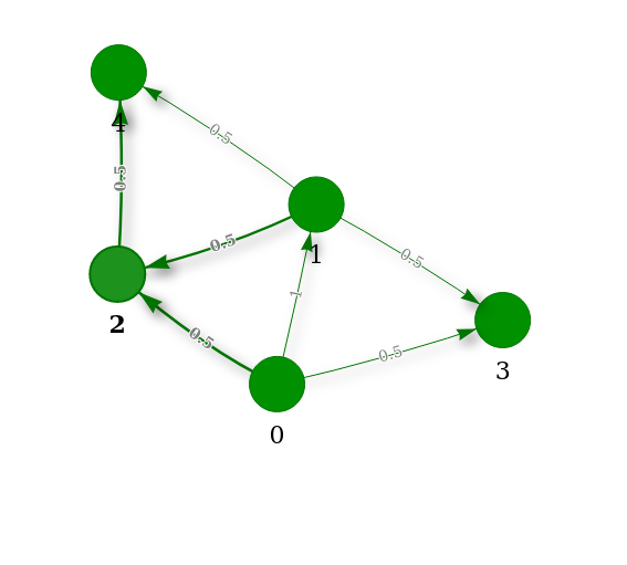
The visualization of a recognition tree looks as follows:

Red nodes indicate dead ends and subtrees without any successful recognition path. In contrast, green leaves and inner nodes indicate metrics on 4 vertices that are R metrics and subtrees with at least one successful path, respectively.

Box graphs

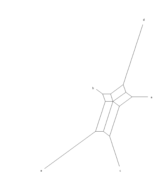
All (pseudo)metrics on four items can be represented by a "box graph". The four items are the leaves, i.e., the vertices with degree one. Their distances are given by the sum of edge lengths of any shortest path.

The sides of the rectangle are r and s. The "spikes" are the edges incident with the leaves x, y, z, and u. Here, the spike of u has length 0.

The function plot_box_graph in the module erdbeermet.visualize.BoxGraphVis takes a distance matrix on four items as input and visualizes it as a box graph:

from erdbeermet.simulation import simulate
from erdbeermet.visualize.BoxGraphVis import plot_box_graph

# simulate scenario on 4 items
scenario = simulate(4)

# plot box graph with custom leaf labels
plot_box_graph(scenario.D, labels=['a', 'b', 'c', 'd'])

References

What are R pseudometrics/matrices?

• Prohaska, S.J., Berkemer, S.J., Gärtner, F., Gatter, T., Retzlaff, N., The Students of the Graphs and Biological Networks Lab 2017, Höner zu Siederdissen, C., Stadler, P.F. (2017) Expansion of gene clusters, circular orders, and the shortest Hamiltonian path problem. Journal of Mathematical Biology. doi: 10.1007/s00285-017-1197-3.