Logistic Regression in the Diagnosis of Parkinson's Disease / Parkinson Hastalığı Tanısında Lojistik Regresyon (tr)

In this notebook we will implement logistic regression to diagnose parkinson disease, the dataset is obtained from Oxford Parkinson's Disease Detection Dataset (https://archive.ics.uci.edu/dataset/174/parkinsons)

Dataset

• This dataset is composed of a range of biomedical voice measurements from 31 people, 23 with Parkinson's disease (PD). Each column in the table is a particular voice measure, and each row corresponds one of 195 voice recording from these individuals ("name" column). The main aim of the data is to discriminate healthy people from those with PD, according to "status" column which is set to 0 for healthy and 1 for PD.

• The data is in ASCII CSV format. The rows of the CSV file contain an instance corresponding to one voice recording. There are around six recordings per patient, the name of the patient is identified in the first column.For further information or to pass on comments, please contact Max Little (littlem '@' robots.ox.ac.uk).

• Here is a brief of the dataset, peeking it using pandas

Reference:

Max A. Little, Patrick E. McSharry, Eric J. Hunter, Lorraine O. Ramig (2008), 'Suitability of dysphonia measurements for telemonitoring of Parkinson's disease', IEEE Transactions on Biomedical Engineering

Data Analyzation

The data analysis phase aims to provide an understanding of the dataset, highlighting key relationships, distributions, and feature types. This knowledge will guide preprocessing steps and contribute to the development of an effective logistic regression model for diagnosing Parkinson's disease.

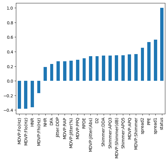
Correlation Analysis:

• Exploring the correlation between each feature and the target variable (status) and identifying features that exhibit a strong correlation, as these may play a significant role in the diagnostic process.

Distribution Analysis:

• Examining the distribution of target variable values (1 and 0) to understand the prevalence of Parkinson's disease in the dataset and identifying potential class imbalances that may impact model training and evaluation.

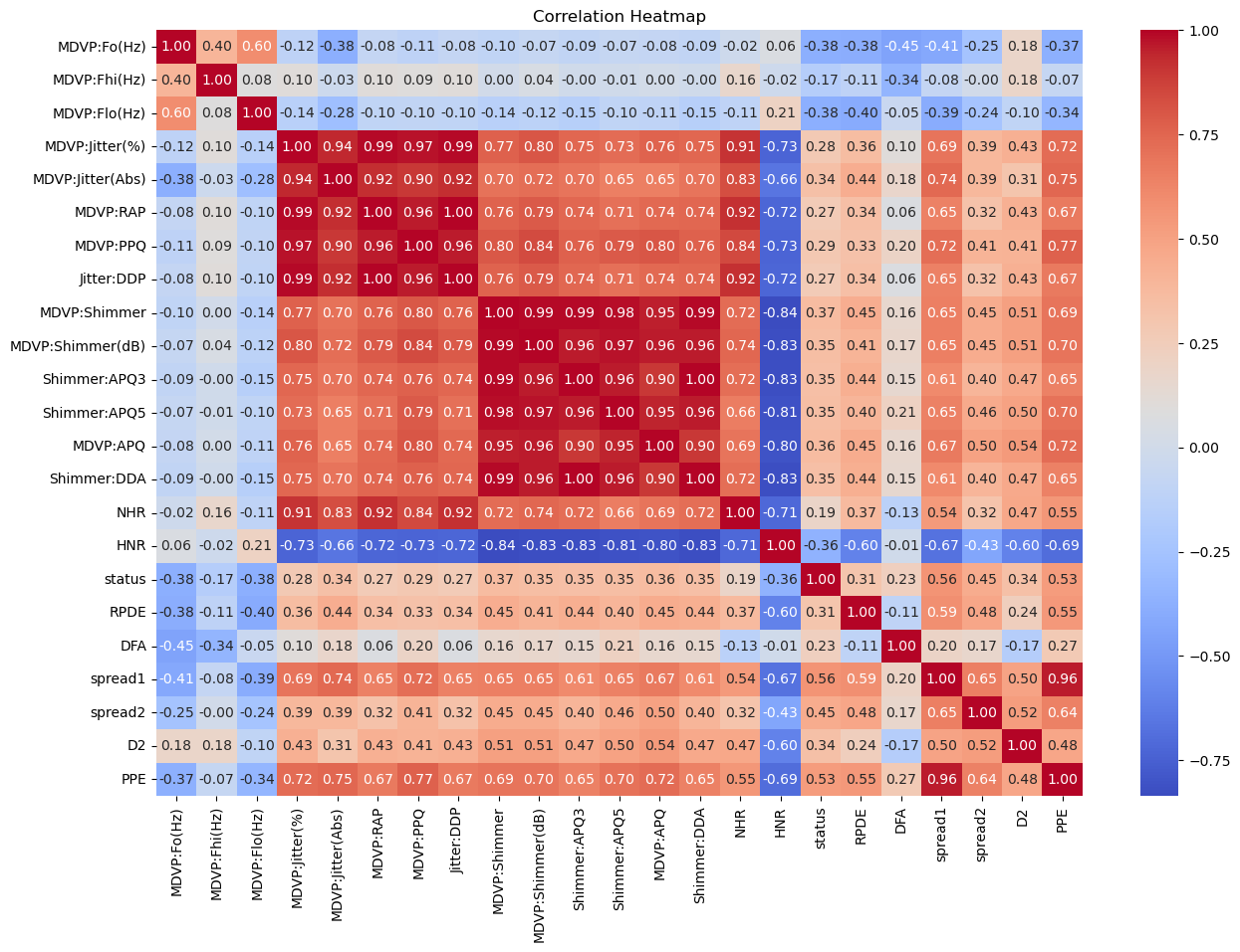
Correlation Heatmap:

• Visualize the correlation matrix of numeric features in the dataset

Logistic Regression

Logistic Regression (also known as logit model) is often used for classification and predictive analytics. Logistic regression estimates the probability of an event occurring. Since the outcome is a probability, the dependent variable is bounded between 0 and 1 which aligns with the case we are dealing with here.

Sigmoid Function

Logistic regression model is represented as

$$ f_{\mathbf{w},b}(x) = g(\mathbf{w}\cdot \mathbf{x} + b)$$

where function $g$ is the sigmoid function. The sigmoid function is defined as:

$$g(z) = \frac{1}{1+e^{-z}}$$

Here is the implementation using Python:

def sigmoid(z):
    """
    Compute the sigmoid of z
    """
    g = 1 / (1 + np.exp(-z))
    
    return g

Cost Function

Logistic regression cost function is of the form

$$ J(\mathbf{w},b) = \frac{1}{m}\sum_{i=0}^{m-1} \left[ loss(f_{\mathbf{w},b}(\mathbf{x}^{(i)}), y^{(i)}) \right] \tag{1}$$

where

• m is the number of training examples in the dataset

• $loss(f_{\mathbf{w},b}(\mathbf{x}^{(i)}), y^{(i)})$ is the cost for a single data point, which is -

  $$loss(f_{\mathbf{w},b}(\mathbf{x}^{(i)}), y^{(i)}) = (-y^{(i)} \log\left(f_{\mathbf{w},b}\left( \mathbf{x}^{(i)} \right) \right) - \left( 1 - y^{(i)}\right) \log \left( 1 - f_{\mathbf{w},b}\left( \mathbf{x}^{(i)} \right) \right) \tag{2}$$

• $f_{\mathbf{w},b}(\mathbf{x}^{(i)})$ is the model's prediction, while $y^{(i)}$, which is the actual label

• $f_{\mathbf{w},b}(\mathbf{x}^{(i)}) = g(\mathbf{w} \cdot \mathbf{x^{(i)}} + b)$ where function $g$ is the sigmoid function.

Here is the implementation using Python:

def compute_cost(X, y, w, b, *argv):
    """
    Computes the cost over all examples
    """

    m, n = X.shape
    cost = 0.
    
    for i in range(m):
        z_i = np.dot(X[i], w) + b
        f_wb_i = sigmoid(z_i)
        cost += - y[i] * np.log(f_wb_i) - (1 - y[i]) * np.log(1 - f_wb_i)

    total_cost = cost / m

    return total_cost

Gradient Descent

Gradient descent algorithm is:

$$\begin{align*}& \text{repeat until convergence:} ; \lbrace \newline ; & b := b - \alpha \frac{\partial J(\mathbf{w},b)}{\partial b} \newline ; & w_j := w_j - \alpha \frac{\partial J(\mathbf{w},b)}{\partial w_j} \tag{1} ; & \text{for j := 0..n-1}\newline & \rbrace\end{align*}$$

where, parameters $b$, $w_j$ are all updated simultaniously

This compute_gradient function is to compute $\frac{\partial J(\mathbf{w},b)}{\partial w}$, $\frac{\partial J(\mathbf{w},b)}{\partial b}$ from equations (2) and (3) below.

$$ \frac{\partial J(\mathbf{w},b)}{\partial b} = \frac{1}{m} \sum\limits_{i = 0}^{m-1} (f_{\mathbf{w},b}(\mathbf{x}^{(i)}) - \mathbf{y}^{(i)}) \tag{2} $$ $$ \frac{\partial J(\mathbf{w},b)}{\partial w_j} = \frac{1}{m} \sum\limits_{i = 0}^{m-1} (f_{\mathbf{w},b}(\mathbf{x}^{(i)}) - \mathbf{y}^{(i)})x_{j}^{(i)} \tag{3} $$

• m is the number of training examples in the dataset

• $f_{\mathbf{w},b}(x^{(i)})$ is the model's prediction, while $y^{(i)}$ is the actual label

Here is the implementation using Python:

def compute_gradient(X, y, w, b, *argv): 
    """
    Computes the gradient for logistic regression  
    """
    m, n = X.shape
    dj_dw = np.zeros(w.shape)
    dj_db = 0.

    for i in range(m):
        z_wb = np.dot(X[i], w) + b
        f_wb = sigmoid(z_wb)
        
        dj_db_i = f_wb - y[i]
        dj_db += dj_db_i
        
        for j in range(n): 
            dj_dw[j] += X[i, j] * dj_db_i
            
    dj_db /= m
    dj_dw /= m
        
    return dj_db, dj_dw