
You can also find all 44 answers here 👉 Devinterview.io - Heap and Map Data Structures
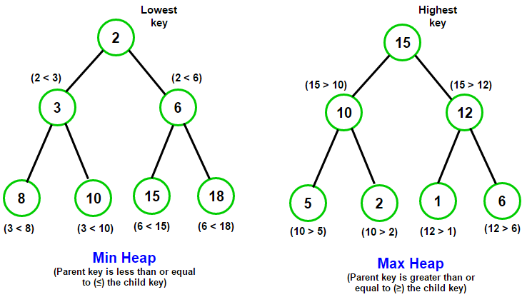
A Heap is a tree-based data structure that is commonly used to implement priority queues. There are two primary types of heaps: Min Heap and Max Heap.
In a Min Heap, the root node is the smallest element, and each parent node is smaller than or equal to its children. Conversely, in a Max Heap, the root node is the largest element, and each parent node is greater than or equal to its children.
- Completeness: All levels of the tree are fully populated except for possibly the last level, which is filled from left to right.
- Heap Order: Each parent node adheres to the heap property, meaning it is either smaller (Min Heap) or larger (Max Heap) than or equal to its children.
The Binary Heap is a popular heap implementation that is essentially a complete binary tree. The tree can represent either a Min Heap or Max Heap, with sibling nodes not being ordered relative to each other.
Binary heaps are usually implemented using an array, where:
- Root:
heap[0] - Left Child:
heap[2 * i + 1] - Right Child:
heap[2 * i + 2] - Parent:
heap[(i - 1) // 2]
- Insert: Adds an element while maintaining the heap order, generally using a "heapify-up" algorithm.
- Delete-Min/Delete-Max: Removes the root and restructures the heap, typically using a "heapify-down" or "percolate-down" algorithm.
- Peek: Fetches the root element without removing it.
- Heapify: Builds a heap from an unordered collection.
- Size: Returns the number of elements in the heap.
-
Insert:
$O(\log n)$ -
Delete-Min/Delete-Max:
$O(\log n)$ -
Peek:
$O(1)$ -
Heapify:
$O(n)$ -
Size:
$O(1)$
Here is the Python code:
# Utility functions for heapify-up and heapify-down
def heapify_up(heap, idx):
    parent = (idx - 1) // 2
    if parent >= 0 and heap[parent] > heap[idx]:
        heap[parent], heap[idx] = heap[idx], heap[parent]
        heapify_up(heap, parent)

def heapify_down(heap, idx, heap_size):
    left = 2 * idx + 1
    right = 2 * idx + 2
    smallest = idx
    if left < heap_size and heap[left] < heap[smallest]:
        smallest = left
    if right < heap_size and heap[right] < heap[smallest]:
        smallest = right
    if smallest != idx:
        heap[idx], heap[smallest] = heap[smallest], heap[idx]
        heapify_down(heap, smallest, heap_size)

# Complete MinHeap class
class MinHeap:
    def __init__(self):
        self.heap = []

    def insert(self, value):
        self.heap.append(value)
        heapify_up(self.heap, len(self.heap) - 1)

    def delete_min(self):
        if not self.heap:
            return None
        min_val = self.heap[0]
        self.heap[0] = self.heap[-1]
        self.heap.pop()
        heapify_down(self.heap, 0, len(self.heap))
        return min_val

    def peek(self):
        return self.heap[0] if self.heap else None

    def size(self):
return len(self.heap)A Priority Queue is a specialized data structure that manages elements based on their assigned priorities. In this queue, higher-priority elements are processed before lower-priority ones.
- Dynamic Ordering: The queue adjusts its order as elements are inserted or their priorities are updated.
- Efficient Selection: The queue is optimized for quick retrieval of the highest-priority element.
- Insert: Adds an element and its associated priority.
- Delete-Max (or Min): Removes the highest-priority element.
- Peek: Retrieves but does not remove the highest-priority element.
-
Insert:
$O(\log n)$ -
Delete-Max (or Min):
$O(\log n)$ -
Peek:
$O(1)$
-
Unsorted Array/List: Quick inserts
$O(1)$ but slower maximum-priority retrieval$O(n)$ . -
Sorted Array/List: Slower inserts
$O(n)$ but quick maximum-priority retrieval$O(1)$ . - Binary Heap: Balanced performance for both insertions and deletions.
Here is the Python code:
import heapq

# Initialize an empty Priority Queue
priority_queue = []

# Insert elements
heapq.heappush(priority_queue, 3)
heapq.heappush(priority_queue, 1)
heapq.heappush(priority_queue, 2)

# Remove and display the highest-priority element
print(heapq.heappop(priority_queue)) # Output: 1Binary heaps can be either a max heap or a min heap. The main difference lies in the heapifying process, where parent nodes either dominate (in a max heap) or are smaller than (in a min heap) their child nodes.
- Ordering: Each node is greater than or equal to its children.
- Visual Representation: The structure looks like an inverted pyramid or an "upside-down tree". The parent nodes are greater than or equal to the child nodes.
       9
     /   \
    5     7
   / \   / \
  4   1 6   3
- Ordering: Each node is less than or equal to its children.
- Visual Representation: The structure looks like a regular "tree", where each parent node is lesser than or equal to its children.
      1
     / \
    2   3
   / \ / \
  9  6 7  8
Both heap types share the following key operations:
- peek: Accesses the root element without deleting it.
- insert: Adds a new element to the heap.
- remove: Removes the root element (top element, or the top priority element in the case of a priority queue).
Heap Property, which distinguishes the heap from an ordinary tree, can be maintained in both Insert and Delete operations.
When a new element is inserted, the upward heapization or bubble-up process is crucial for preserving the heap property.

Here is the Python code:
# Upward heapify on insertion
def heapify_upwards(heap, i):
    parent = (i - 1) // 2
    if parent >= 0 and heap[parent] < heap[i]:
        heap[parent], heap[i] = heap[i], heap[parent]
        heapify_upwards(heap, parent)

def insert_element(heap, element):
    heap.append(element)
heapify_upwards(heap, len(heap) - 1)Whether it's a Max Heap or Min Heap, the downward heapification or trickle-down process is employed for maintaining the heap property after a deletion.

Here is the Python code for a Max Heap:
# Downward heapify on deletion
def heapify_downwards(heap, i):
    left_child = 2 * i + 1
    right_child = 2 * i + 2
    largest = i

    if left_child < len(heap) and heap[left_child] > heap[largest]:
        largest = left_child
    if right_child < len(heap) and heap[right_child] > heap[largest]:
        largest = right_child

    if largest != i:
        heap[i], heap[largest] = heap[largest], heap[i]
        heapify_downwards(heap, largest)

def delete_max(heap):
    heap[0], heap[-1] = heap[-1], heap[0]
    deleted_element = heap.pop()
    heapify_downwards(heap, 0)
return deleted_element-
Time Complexity:
$O(\log n)$ for both insert and delete as these operations are backed by heapify_upwards and heapify_downwards, both of which have logarithmic time complexities in a balanced binary tree. -
Space Complexity:
$O(1)$ for both insert and delete as they only require a constant amount of extra space.
Suppose we have a binary heap represented as follows:
        77
       /  \
      50   60
     / \   / \
    22  30 44  55
The task is to insert the value 55 into this binary heap while maintaining its properties.
- Adding the Element to the Bottom Level: Initially, the element is placed at the next available position in the heap to maintain the heap's shape property.
- Heapify-Up: The element is then moved up the tree until it is in the correct position, satisfying both the shape property and the heap property. This process is often referred to as "sift-up" or "bubble-up".
Let's walk through the steps for inserting 55 into the above heap.
Step 1: Add the Element to the Bottom Level
The next available position, following the shape property, is the first empty spot in the heap, starting from the left. The element 55 will go to the left of 22 in this case.
        77
       /  \
      50   60
     / \   / \
    22  30 44  55
    /
   55
Step 2: Heapify-Up
We start the heapify-up process from the newly added element and move it up through the heap as needed.
- Compare
55with its parent22. Since55 > 22, they are swapped.
        77
       /  \
      50   60
     / \   / \
    55  30 44  22
    /
   55
- Now, compare the updated element
55with its new parent50. As55 > 50, they are swapped.
        77
       /  \
      55   60
     / \   / \
    50  30 44  22
    /
   55
- Finally, compare
55with its parent77. As55 < 77, no more swapping is needed, and we can stop.
Final Heap
The final heap looks like this:
        77
       /  \
      55   60
     / \   / \
    50  30 44  22
    /
   55
Here is the Python code:
import heapq

# Initial heap
heap = [77, 50, 60, 22, 30, 44, 55]

# Add the new element
heap.append(55)

# Perform heapify-up
heapq._siftdown(heap, 0, len(heap)-1)

print("Final heap:", heap)
The output will be:
Final heap: [77, 55, 60, 22, 30, 44, 50, 55]
This final heap is a Min-Heap, as we used the _siftdown function from the heapq module, which is designed for Min-Heaps.
Let's compare arrays and binary heap data structures used for implementing a priority queue in terms of their algorithms and performance characteristics.
- Array-Based: An unsorted or sorted list where the highest-priority element is located via a linear scan.
- Binary Heap-Based: A binary tree with special properties, ensuring efficient access to the highest-priority element.
-
Array-Based:
- getMax:
$O(n)$ - insert:
$O(1)$ - deleteMax:
$O(n)$
- getMax:
-
Binary Heap-Based:
- getMax:
$O(1)$ - insert:
$O(\log n)$ - deleteMax:
$O(\log n)$
- getMax:
-
Array-Based:
- Small datasets: If the dataset size is small or the frequency of
getMaxanddeleteMaxoperations is low, an array can be a simpler and more direct choice. - Memory considerations: When working in environments with very constrained memory, the lower overhead of a static array might be beneficial.
- Predictable load: If the primary operations are insertions and the number of
getMaxordeleteMaxoperations is minimal and predictable, an array can suffice.
- Small datasets: If the dataset size is small or the frequency of
-
Binary Heap-Based:
- Dynamic datasets: If elements are continuously being added and removed, binary heaps provide more efficient operations for retrieving and deleting the max element.
- Larger datasets: Binary heaps are more scalable and better suited for larger datasets due to logarithmic complexities for insertions and deletions.
- Applications demanding efficiency: For applications like task scheduling systems, network packet scheduling, or algorithms like Dijkstra's and Prim's, where efficient priority operations are crucial, binary heaps are the preferred choice.
Here is the Python code:
class ArrayPriorityQueue:
    def __init__(self):
        self.array = []

    def getMax(self):
        return max(self.array)

    def insert(self, item):
        self.array.append(item)

    def deleteMax(self):
        max_val = self.getMax()
        self.array.remove(max_val)
return max_valHere is the Python code:
import heapq

class BinaryHeapPriorityQueue:
    def __init__(self):
        self.heap = []

    def getMax(self):
        return -self.heap[0]  # Max element will be at the root in a max heap

    def insert(self, item):
        heapq.heappush(self.heap, -item)

    def deleteMax(self):
return -heapq.heappop(self.heap)For modern applications, using library-based priority queue implementations is often the best choice. They are typically optimized and built upon efficient data structures like binary heaps.
Dynamic arrays, or vectors, provide a more memory-efficient representation of heaps compared to static arrays.
-
Amortized
$O(1)$ Insertions and Deletions. This holds until resizing is necessary. - Memory Flexibility. They can shrink, unlike static arrays. This means you won't waste memory with an over-allocated heap.
-
Insertion. Place the new element at the end and then "sift up", swapping with its parent until the heap property is restored.
-
Deletion. Remove the root (which is the minimum in a min-heap), replace it with the last element, and then "sift down", comparing with children and swapping, ensuring the heap is valid.
Here is the Python code:
class DynamicArrayMinHeap:
    def __init__(self):
        self.heap = []

    def parent(self, i):
        return (i - 1) // 2

    def insert(self, val):
        self.heap.append(val)
        self._sift_up(len(self.heap) - 1)

    def extract_min(self):
        if len(self.heap) == 0:
            return None

        if len(self.heap) == 1:
            return self.heap.pop()

        min_val = self.heap[0]
        self.heap[0] = self.heap.pop()
        self._sift_down(0)
        return min_val

    def _sift_up(self, i):
        while i > 0 and self.heap[i] < self.heap[self.parent(i)]:
            self.heap[i], self.heap[self.parent(i)] = self.heap[self.parent(i)], self.heap[i]
            i = self.parent(i)

    def _sift_down(self, i):
        smallest = i
        left = 2 * i + 1
        right = 2 * i + 2

        if left < len(self.heap) and self.heap[left] < self.heap[smallest]:
            smallest = left
        if right < len(self.heap) and self.heap[right] < self.heap[smallest]:
            smallest = right

        if smallest != i:
            self.heap[i], self.heap[smallest] = self.heap[smallest], self.heap[i]
self._sift_down(smallest)- Time-Sensitive Applications. If time-efficiency is crucial and long waits for array expansions are not acceptable, dynamic arrays are a better choice.
- Databases. Dynammic arrays are often used for memory management by database systems to handle variable-length fields in records more efficiently.
Let's look at different ways Priority Queues can be implemented and the time complexities associated with each approach.
-
Unordered List:
- Insertion:
$O(1)$ - Deletion/Find Min/Max:
$O(n)$
- Insertion:
-
Ordered List:
- Insertion:
$O(n)$ - Deletion/Find Min/Max:
$O(1)$
- Insertion:
-
Unordered Array:
- Insertion:
$O(1)$ - Deletion/Find Min/Max:
$O(n)$
- Insertion:
-
Ordered Array:
- Insertion:
$O(n)$ - Deletion/Find Min/Max:
$O(1)$
- Insertion:
-
Binary Search Tree (BST):
- All Operations:
$O(\log n)$ (can degrade to$O(n)$ if unbalanced)
- All Operations:
-
Balanced BST (e.g., AVL Tree):
- All Operations:
$O(\log n)$
- All Operations:
-
Binary Heap:
- Insertion/Deletion:
$O(\log n)$ - Find Min/Max:
$O(1)$
- Insertion/Deletion:
Lazy deletion keeps the deletion process simple, optimizing for both time and space efficiency. The primary goal is to reduce the number of "holes" in the heap to minimize reordering operations.
When you remove an item:
- The item to be removed is tagged as deleted, marking it as a "hole" in the heap.
- The heap structure is restored without actively swapping the item with the last element.
- Efficiency: Reduces the noticeable overhead that can come with extensive restructuring.
- Simplicity: Provides a straightforward algorithm for the removal process, which aligns well with the rigidity and set rules of a heap.
-
Time Complexity: While operations like
removeMin$orremoveMax$ remain O$log n$, the actual time complexity can be slightly higher than that, as the algorithm potentially takes more time when it encounters a hole. - "Hole" Management: Too many "holes" can degrade performance, necessitating eventual cleanup.
Here is the Python code:
class LazyDeletionHeap(MinHeap):
    def __init__(self):
        super().__init__()
        self.deleted = set()

    def delete(self, item):
        if item in self.array:
            self.deleted.add(item)

    def remove_min(self):
        while self.array and self.array[0] in self.deleted:
            self.deleted.remove(self.array[0])
            self.array.pop(0)
            self.heapify()
        if self.array:
            return self.array.pop(0)
In this code, minHeap is a normal heap structure, and array is the list used to represent the heap indexing starts from 0.
Heapify is a method that ensures the heap property is maintained for a given array, typically performed in the background during heap operations.
Without Heapify, operations like insert or delete on heaps can take up to
The starting point is usually the bottom-most, rightmost "subtree" of the heap.
-
Locate:
- Identify the multi-level rightmost leaf of the subtree.
-
Sift Upwards: Peform a parent-child comparison in binary heaps to correct the heap order.
- If the child node is greater (for a max heap), swap it with the parent.
- Repeat this process, moving upwards, until the parent is greater than both its children or until the root is reached.
-
Repeat:
- Continue the process sequentially for each level, from right to left.
Focused on the local structure, this process simplifies the task to
-
Time Complexity:
$O(\log n)$ -
Space Complexity:
$O(1)$
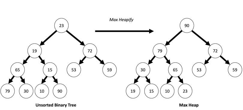
In the example above, we begin heapifying from the right-bottom node (index 6), compare it with its parent (index 2) and move upwards, ensuring the max-heap property is satisfied.
Here is the Python code:
def heapify(arr, n, i):
    largest = i
    l = 2 * i + 1
    r = 2 * i + 2

    if l < n and arr[i] < arr[l]:
        largest = l

    if r < n and arr[largest] < arr[r]:
        largest = r

    if largest != i:
        arr[i], arr[largest] = arr[largest], arr[i]
        heapify(arr, n, largest)

# Example usage to build a max heap
arr = [12, 11, 10, 5, 6, 2, 1]
n = len(arr)
for i in range(n//2 - 1, -1, -1):
heapify(arr, n, i)Heap Sort is a robust comparison-based sorting algorithm that uses a binary heap data structure to build a "heap tree" and then sorts the elements.
- Selection-Based: Iteratively selects the largest (in a max heap) or the smallest (in a min heap) element.
-
In-Place: Sorts the array within its original storage without the need for additional memory, yielding a space complexity of
$O(1)$ . - Unstable: Does not guarantee the preservation of the relative order of equal elements.
- Less Adaptive: Doesn't take advantage of existing or partial order in a dataset.
- Heap Construction: Transform the input array into a max heap.
- Element Removal: Repeatedly remove the largest element from the heap and reconstruct the heap.
- Array Formation: Place the removed elements back into the array in sorted order.
-
Time Complexity: Best, Average, and Worst Case:
$O(n \log n)$ - Building the heap is$O(n)$ and each of the$n$ removals requires$\log n$ time. -
Space Complexity:
$O(1)$
Here is the Python code:
def heapify(arr, n, i):
    largest = i
    l = 2 * i + 1
    r = 2 * i + 2

    if l < n and arr[l] > arr[largest]:
        largest = l
    if r < n and arr[r] > arr[largest]:
        largest = r
    if largest != i:
        arr[i], arr[largest] = arr[largest], arr[i]
        heapify(arr, n, largest)

def heap_sort(arr):
    n = len(arr)
    for i in range(n // 2 - 1, -1, -1):
        heapify(arr, n, i)
    for i in range(n-1, 0, -1):
        arr[i], arr[0] = arr[0], arr[i]
        heapify(arr, i, 0)
return arrLet's discuss a novel and a traditional sorting algorithm and their respective performance characteristics.
-
Time Complexity:
- Best & Average:
$O(n \log n)$ - Worst:
$O(n^2)$ - when the pivot choice is consistently bad, e.g., always selecting the smallest or largest element.
- Best & Average:
-
Expected Space Complexity: O(
$\log n$ ) - In-place algorithm. - Partitioning: Efficient for large datasets with pivot selection and partitioning.
-
Time Complexity:
- Best, Average, Worst:
$O(n \log n)$ - consistent behavior regardless of data.
- Best, Average, Worst:
-
Space Complexity:
$O(1)$ - In-place algorithm. -
Heap Building:
$O(n)$ - extra initial step to build the heap. - Stability: May become unstable after initial build, unless modifications are made.
- External Data Buffer: Maintains data integrity during the sorting process, leading to its widespread use in numerous domains.
To merge
-
Initialize: Build a min-heap of size
$k$ with the first element of each array. - Iterate: Remove the minimum from the heap, add the next element of its array to the heap if available, and repeat until the heap is empty.
- Complete: The heap holds the smallest remaining elements, output these in order.
-
Time Complexity:
$O(n \cdot \log k)$ - Both building the initial heap and each element removal and insertion takes$O(\log k)$ time. -
Space Complexity:
$O(k)$ - The heap can contain at most$k$ elements.
Here is the Python code:
import heapq

def merge_k_sorted_arrays(arrays):
    result = []

    # Initialize min-heap with first element from each array
    heap = [(arr[0], i, 0) for i, arr in enumerate(arrays) if arr]
    heapq.heapify(heap)

    # While heap is not empty, keep track of minimum element
    while heap:
        val, array_index, next_index = heapq.heappop(heap)
        result.append(val)
        next_index += 1
        if next_index < len(arrays[array_index]):
            heapq.heappush(heap, (arrays[array_index][next_index], array_index, next_index))

    return result

# Example usage
arrays = [[1, 3, 5], [2, 4, 6], [0, 7, 8, 9]]
merged = merge_k_sorted_arrays(arrays)
print(merged) # Output: [0, 1, 2, 3, 4, 5, 6, 7, 8, 9]The goal is to build a data structure, representing either a min or max heap, that supports efficient find operations for both the minimum and maximum elements within the heap.
To fulfill the Find-Min and Find-Max requirements, two heaps are used in tandem:
- A
Min-Heapensures the minimum element can be quickly retrieved, with the root holding the smallest value. - A
Max-Heapfacilitates efficient access to the maximum element, positioning the largest value at the root.
The overall time complexity for both find operations is
- Initialize Both Heaps: Choose the appropriate built-in library or implement the heap data structure. Here, we'll use the
heapqlibrary in Python. - Insert Element: With a single heap, inserting an element only involves pushing it onto the heap. However, with two heaps, each new element needs to be placed on the heap that will balance the size. This ensures that the root of one heap will correspond to the minimum or maximum value across all elements.
- Retrieve Min & Max: For both operations, simply access the root of the corresponding heap.
-
Time Complexity:
-
findMinandfindMax:$O(1)$ -
insert:$O(\log n)$
-
-
Space Complexity:
$O(n)$ for both heaps.
Here is the code:
import heapq

class FindMinMaxHeap:
    def __init__(self):
        self.min_heap, self.max_heap = [], []
        self.size = 0

    def insert(self, num):
        if self.size % 2 == 0:
            heapq.heappush(self.max_heap, -1 * num)
            self.size += 1
            if len(self.min_heap) == 0:
                return
            if -1 * self.max_heap[0] > self.min_heap[0]:
                max_root = -1 * heapq.heappop(self.max_heap)
                min_root = heapq.heappop(self.min_heap)
                heapq.heappush(self.max_heap, -1 * min_root)
                heapq.heappush(self.min_heap, max_root)
        else:
            if num < -1 * self.max_heap[0]:
                heapq.heappush(self.min_heap, -1 * heapq.heappop(self.max_heap))
                heapq.heappush(self.max_heap, -1 * num)
            else:
                heapq.heappush(self.min_heap, num)
            self.size += 1

    def findMin(self):
        if self.size % 2 == 0:
            return (-1 * self.max_heap[0] + self.min_heap[0]) / 2.0
        else:
            return -1 * self.max_heap[0]

    def findMax(self):
        if self.size % 2 == 0:
            return (-1 * self.max_heap[0] + self.min_heap[0]) / 2.0
        else:
            return -1 * self.max_heap[0]

# Example
mmh = FindMinMaxHeap()
mmh.insert(3)
mmh.insert(5)
print("Min:", mmh.findMin())  # Output: 3
print("Max:", mmh.findMax())  # Output: 5
mmh.insert(1)
print("Min:", mmh.findMin())  # Output: 2
print("Max:", mmh.findMax()) # Output: 3Heaps find application in a variety of algorithms and data handling tasks.
-
Extreme Value Access: The root of a min-heap provides the smallest element, while the root of a max-heap provides the largest, allowing constant-time access.
-
Selection Algorithms: Heaps can efficiently find the
$k^{th}$ smallest or largest element in$O(k \log k + n)$ time. -
Priority Queue: Using heaps, we can effectively manage a set of data wherein each element possesses a distinct priority, ensuring operations like insertion, maximum extraction, and sorting are performed efficiently.
-
Sorting: Heaps play a pivotal role in the Heap Sort algorithm, offering
$O(n \log n)$ time complexity. They're also behind utility functions in some languages likenlargest()andnsmallest(). -
Merge Sorted Streams: Heaps facilitate the merging of multiple pre-sorted datasets or streams into one cohesive sorted output.
-
Graph Algorithms: Heaps, especially when implemented as priority queues, are instrumental in graph algorithms such as Dijkstra's Shortest Path and Prim's Minimum Spanning Tree, where they assist in selecting the next node to process efficiently.
Explore all 44 answers here 👉 Devinterview.io - Heap and Map Data Structures