Top 70 Ensemble Learning Interview Questions

You can also find all 70 answers here 👉 Devinterview.io - Ensemble Learning

1. What is ensemble learning in machine learning?

Ensemble learning involves combining multiple machine learning models to yield stronger predictive performance. This collaborative approach is particularly effective when individual models are diverse yet competent.

Key Characteristics

• Diversity: Models should make different kinds of mistakes and have distinct decision-making mechanisms.
• Accuracy & Consistency: Individual models, known as "weak learners," should outperform randomness in their predictions.

Benefits

• Performance Boost: Ensembles often outperform individual models, especially when those models are weak learners.
• Robustness: By aggregating predictions, ensembles can be less sensitive to noise in the data.
• Generalization: They can generalize well to new, unseen data.
• Reduction of Overfitting: Combining models can help reduce overfitting.

Common Ensemble Methods

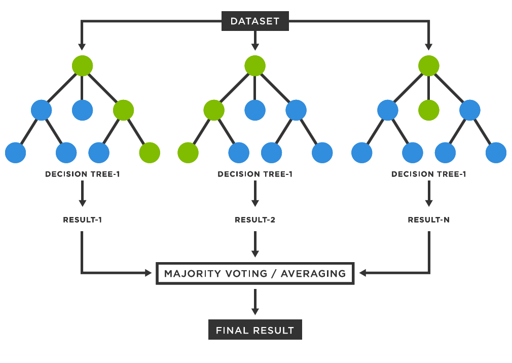
• Bagging: Trains models on data subsets, using a combination (such as a majority vote or averaging) to make predictions.
• Boosting: Trains models sequentially, with each subsequent model learning from the mistakes of its predecessor.
• Stacking: Employs a "meta-learner" to combine predictions made by base models.

Ensuring Model Diversity

• Data Sampling: Use different subsets for different models.
• Feature Selection: Train models on different subsets of features.
• Model Selection: Utilize different types of models with varied strengths and weaknesses.

Core Concepts

Voting

• Task: Each model makes a prediction, and the most common prediction is chosen.
• Types:
  • Hard Voting: Majority vote. Suitable for classification.
  • Soft Voting: Probabilistic average. Appropriate for both classification and regression.

Averaging

• Task: Models generate predictions, and the mean (or another statistical measure) is taken.
• Types:
  • Simple Averaging: Straightforward mean calculation.
  • Weighted Averaging: Assigns individual model predictions different importance levels.

Stacking

• Task: Combines predictions from multiple models using a meta-learner, often a more sophisticated model like a neural network.

Code Example: Majority Voting

Here is the Python code:

from statistics import mode

# Dummy predictions from individual models
model1_pred = [0, 1, 0, 1, 1]
model2_pred = [1, 0, 1, 1, 0]
model3_pred = [0, 0, 0, 1, 0]

# Perform majority voting
majority_voted_preds = [mode([m1, m2, m3]) for m1, m2, m3 in zip(model1_pred, model2_pred, model3_pred)]

print(majority_voted_preds)  # Expected output: [0, 0, 0, 1, 0]

Practical Applications for Ensemble Learning

• Kaggle Competitions: Many winning solutions are ensemble-based.
• Financial Sector: For risk assessment, fraud detection, and stock market prediction.
• Healthcare: Especially for diagnostics and drug discovery.
• Remote Sensing: Useful in Earth observation and remote sensing for environmental monitoring.
• E-commerce: For personalized recommendations and fraud detection.

2. Can you explain the difference between bagging, boosting, and stacking?

Bagging, Boosting, and Stacking are all ensemble learning techniques designed to improve model performance, each operating with different methods and algorithms.

Bagging

Bagging uses parallel processing to build multiple models and then aggregates their predictions, usually through majority voting or averaging. Random Forest is a popular example of a bagging algorithm, employing decision trees.

Key Mechanics

• Bootstrap Aggregating: Uses resampling, or "bootstrapping," to create multiple datasets for training.
• Parallel Model Building: Each dataset is used to train a separate model simultaneously.

Code Example: Random Forest

Here is the Python code:

from sklearn.ensemble import RandomForestClassifier

# Create a Random Forest classifier
rf_classifier = RandomForestClassifier(n_estimators=100)

# Train the classifier
rf_classifier.fit(X_train, y_train)

# Make predictions
y_pred_rf = rf_classifier.predict(X_test)

Boosting

Boosting employs a sequential approach where each model corrects the errors of its predecessor. Rather than equal representation, instances are weighted based on previous misclassifications. Adaboost (Adaptive Boosting) and Gradient Boosting Machines (GBM) are classic examples of boosting algorithms.

Key Mechanics

• Weighted Sampling: Misclassified instances are given higher weights to focus on in subsequent training rounds.
• Sequential Model Building: Models are developed one after the other, with each trying to improve the errors of the previous one.

Code Example: Adaboost

Here is the Python code:

from sklearn.ensemble import AdaBoostClassifier

# Create an AdaBoost classifier
ab_classifier = AdaBoostClassifier(n_estimators=100)

# Train the classifier
ab_classifier.fit(X_train, y_train)

# Make predictions
y_pred_ab = ab_classifier.predict(X_test)

Stacking

In contrast to bagging and boosting methods, stacking leverages multiple diverse models, but instead of combining them using majority voting or weighted averages, it adds a meta-learner that takes the predictions of the base models as inputs.

Key Mechanics

• Base Model Heterogeneity: Aim for maximum diversity among base models.
• Meta-Model Training on Base Model Predictions: A meta-model is trained on the predictions of the base models, effectively learning to combine their outputs optimally.

Code Example: Stacking

Here is the Python code:

from sklearn.ensemble import StackingClassifier
from sklearn.linear_model import LogisticRegression

# Create a stacking ensemble with base models (e.g., RandomForest, AdaBoost) and a meta-model (e.g., Logistic Regression)
stacking_classifier = StackingClassifier(
    estimators=[('rf', rf_classifier), ('ab', ab_classifier)],
    final_estimator=LogisticRegression()
)

# Train the stacking classifier
stacking_classifier.fit(X_train, y_train)

# Make predictions
y_pred_stacking = stacking_classifier.predict(X_test)

Common Elements

All three techniques, bagging, boosting, and stacking, share the following characteristics:

• Use of Multiple Models: They incorporate predictions from multiple models, aiming to reduce overfitting and enhance predictive accuracy through model averaging or weighted combinations.
• Data Sampling: They often utilize techniques such as boostrapping or weighted data sampling to present diversity to the individual models.
• Reduced Variance: They help to overcome variance-related issues, like overfitting in individual models, which is valuable when working with limited data.

3. Describe what a weak learner is and how it's used in ensemble methods.

Weak learners in ensemble methods are models that perform only slightly better than random chance, often seen in practice as having 50-60% accuracy. Even with their modest performance, weak learners can be valuable building blocks in creating highly optimized and accurate ensemble models.

Mathematical Framework

Let's assume the given models are decision stumps, i.e., decision trees with only a single split.

A weak learner in the context of decision stumps:

• Has a better-than-random (but still modest) classification performance, typically above 50%.
• The margin of performance, defined as the probability of correct classification minus 0.5, is greater than 0 but relatively small.

A strong learner, in contrast, has a classification rate typically closer to 90% or better, with a larger margin.

Why Weak Learners Are Used

• Robustness: Weak learners are less prone to overfitting, ensuring better generalization to new, unseen data.

• Complementary Knowledge: Each weak learner may focus on a different aspect or subset of the data, collectively providing a more comprehensive understanding.

• Computational Efficiency: Weak learners can often be trained faster than strong learners, making them ideal for large datasets.

• Adaptability: Weak learners can be updated or 'boosted' iteratively, remaining effective as the ensemble model evolves.

Ensemble Techniques That Use Weak Learners

1. Boosting Algorithms: Such as AdaBoost and XGBoost, which sequentially add weak learners and give more weight to misclassified data points.

2. Random Forest: This uses decision trees as its base model. Though decision trees can be strong learners, when they are used as constituents of a random forest, they are 'decorrelated', resulting in a collection of weak learners.

3. Bagging Algorithms: Like Boostrap aggregating, which uses weak learners in the form of decision trees to construct the base estimators.

4. What are some advantages of using ensemble learning methods over single models?

Ensemble Learning combines multiple models to make more accurate predictions. This approach often outperforms using a single model. Below are the key advantages of ensemble learning.

Advantages of Ensemble Learning

1. Increased Accuracy: The amalgamation of diverse models can correct individual model limitations, leading to more accurate predictions.

2. Improved Generalization: Ensemble methods average out noise and potential overfitting, providing better performance on new, unseen data.

3. Enhanced Stability: By leveraging several models, the ensemble is less prone to "wild" predictions from a single model, improving its stability.

4. Robustness to Outliers and Noisy Data: Many ensemble methods, such as Random Forests, are designed to be less affected by outliers and noise.

5. Effective Feature Selection: Features that are consistently useful for prediction across various models in the ensemble are identified as important, aiding in efficient feature selection.

6. Built-in Cross-Validation: Methods like bagging automatically perform internal cross-validation, which can lead to better model assessment and selection.

7. Adaptability to Problem Context: Ensembles can deploy different models based on the problem, such as regression for numerical predictions and classification for categories.

8. Balance of Biases and Variances: Through a careful blend of model types and decision-making mechanisms, ensemble methods can strike a balance between bias and variance. This is particularly true for methods like AdaBoost.

9. Flexibility in Model Choice: Ensemble methods can incorporate various types of models, allowing for robust performance even when specific models may fall short.

10. Wide Applicability: Ensemble methods have proven effective in diverse areas such as finance, healthcare, and natural language processing, among others.

5. How does ensemble learning help with the variance and bias trade-off?

Ensemble learning, through techniques like bagging and boosting, helps to manage the bias-variance tradeoff, offering more predictive power than individual models.

Bias-Variance Tradeoff

• When a model is too simple (high bias), it may not capture the underlying patterns in the data, leading to underfitting.
• On the other hand, when a model is overly complex (high variance), it might fit too closely to the training data and fail to generalize with new data, leading to overfitting.

Ensemble Techniques and Bias-Variance Tradeoff

• Bagging (Bootstrap Aggregating): Uses several models, each trained on a different subset of the dataset, reducing model variance.
• Boosting: Focuses on reducing model bias by sequentially training new models to correct misclassifications made by the existing ensemble.

By figuring out the answer, the confusion about the trade-off between bias and variance gets reduced, leading to a more accurate model.

Bagging and Random Forests

• Bagging: The idea motivats to combine predictions from multiple models (often decision trees). By voting or averaging those results, overfitting is minimized and predictions are more robust.
• Random Forest: This is a more sophisticated version, where each decision tree is trained on a random subset of the features, further reducing correlation between individual trees, and hence, overfitting.

Code Example: Random Forest on Iris Dataset

Here is the Python code:

from sklearn.ensemble import RandomForestClassifier
from sklearn.datasets import load_iris
from sklearn.model_selection import train_test_split
from sklearn.metrics import accuracy_score

# Load dataset
iris = load_iris()
X, y = iris.data, iris.target

# Split the dataset
X_train, X_test, y_train, y_test = train_test_split(X, y, test_size=0.2, random_state=42)

# Create and fit a random forest classifier
rf_model = RandomForestClassifier(n_estimators=100, random_state=42)
rf_model.fit(X_train, y_train)

# Make predictions
y_pred = rf_model.predict(X_test)

# Evaluate accuracy
accuracy = accuracy_score(y_test, y_pred)
print(f"Random Forest Accuracy: {accuracy}")

Here, n_estimators=100 specifies the number of trees in the forest.

6. What is a bootstrap sample and how is it used in bagging?

The bootstrap method is a resampling technique used in machine learning to improve the stability and accuracy of models, especially within ensemble methods.

Why Bootstrap?

Traditional model training uses a single set of data to fit a model, which can be subject to sampling error and instability due to the random nature of the data. Bootstrapping alleviates this by creating multiple subsets through random sampling with replacement.

The Bootstrap Process

• Sample Creation: For a dataset of size $n$, multiple subsets of the same size are created through random sampling with replacement. This means some observations are included multiple times, while others might not be selected at all.

• Model Fitting: Each subset is used to train a separate instance of the model. The resulting models benefit from the diversity introduced by the different subsets, leading to a more robust and accurate ensemble.

Code Example: Bootstrap Sample

Here is the Python code:

import numpy as np

# Create a simple dataset
dataset = np.arange(1, 11)

# Set the seed for reproducibility
np.random.seed(42)

# Generate a bootstrap sample
bootstrap_sample = np.random.choice(dataset, size=10, replace=True)

7. Explain the main idea behind the Random Forest algorithm.

Random Forest is a powerful supervised learning technique that belongs to the category of ensemble methods. This methodology leverages the wisdom of crowds, where multiple decision trees contribute to a more robust prediction, often outperforming individual trees.

The Core Concept: Weighted Majority Vote

Random Forest employs a strategy called majority vote or majority weighted voting.When making a prediction or classification, each decision tree in the forest contributes its input, and the final outcome is determined based on the majority.

• Regression: For a regression task, the individual tree predictions are averaged to obtain the final prediction.

• Classification: Each tree "votes" for a class label, and the class that receives the majority of votes is selected.

Introducing Decision Trees as Clowns

Every decision tree in a Random Forest can be viewed as a slightly quirky clown, characterized by its unique "personality." Despite these individualistic quirks, each tree contributes an essential element to the ensemble, resulting in a cohesive and well-orchestrated performance.

For instance, imagine a circus show where multiple clowns are juggling. Some might occasionally drop the ball, but the majority is skilled enough to keep the "act," i.e., the predictions, on track.

Benefits and Properties

• Robustness: The collective decision-making tends to be more reliable than the output of any single decision tree. Random Forests are particularly effective in noise-ridden datasets.

• Feature Independence: Trees are created using random subsets of features, necessitating each tree to focus on distinctive attributes. This helps in counteracting feature correlations.

• Intrinsic Validation: The out-of-bag (OOB) samples facilitate internal cross-validation, eliminating the need for a separate validation set in some scenarios.

• Feature Importance: The average depth at which a feature is utilized across trees offers insights into its relevance.

• Efficiency: These forests can also be trained in parallel.

Side Notes

• Prediction Speed: While model predictions tend to be rapid, the training procedure can be computationally intensive.

• Memory Consumption: Random Forests can necessitate significant memory, especially in the presence of numerous trees and substantial datasets.

8. How does the boosting technique improve weak learners?

Boosting is an ensemble learning method that improves the accuracy of weak learners. It works by combining the most successful models in a sequential manner, with each subsequent model correcting the errors of its predecessors.

Key Concepts

• Weighted Training: At each iteration, incorrectly classified instances are assigned higher weights for the subsequent model to focus on them.

• Model Agnosticism: Boosting is versatile and can employ any modeling technique as its base classifier, generally referred to as the "weak learner."

• Sequential Learning: Unlike bagging-based techniques such as Random Forest, boosting methods are not easily parallelizable because each model in the sequence relies on the previous models.

Visual Example: AdaBoost

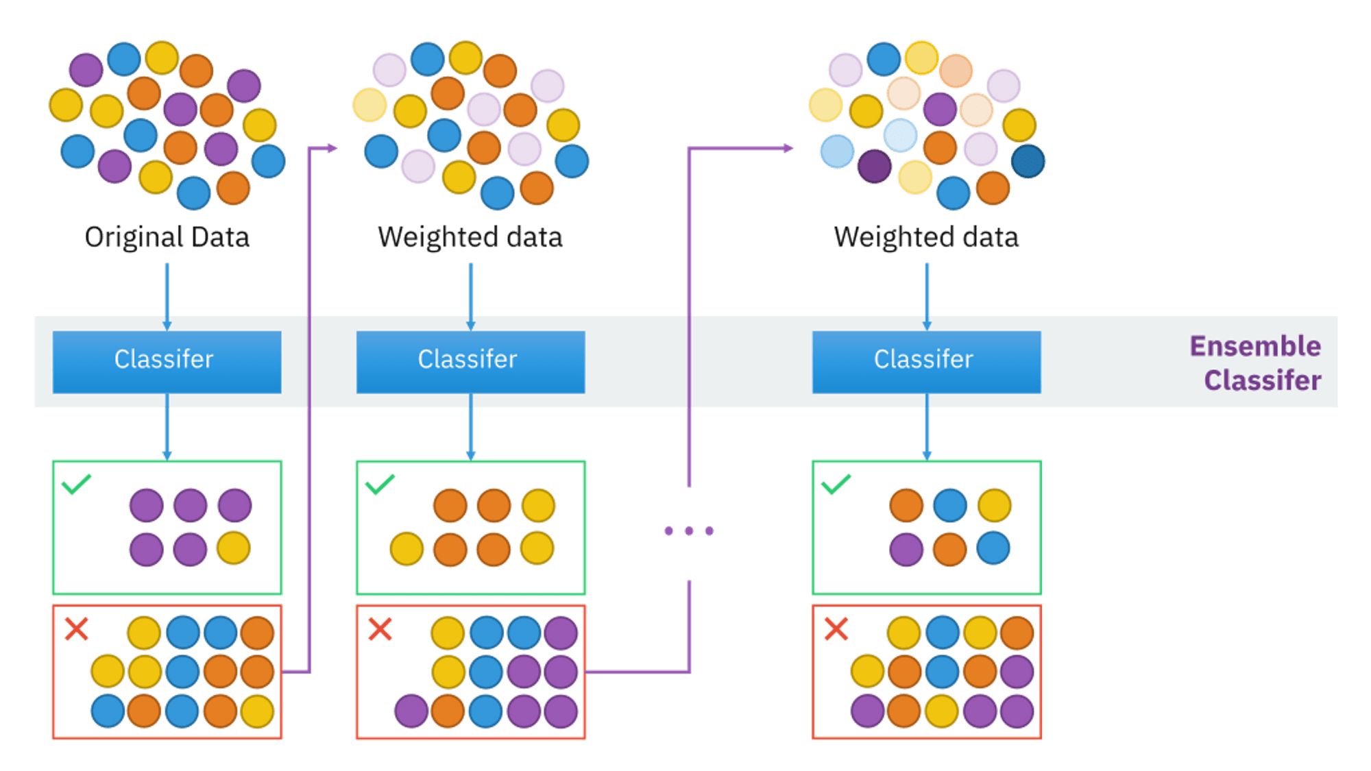
The visual shows how AdaBoost assigns weights to training instances. Misclassified instances (red numbers) receive higher weights (e.g., 27 is updated to 37, and 7 to 23) to become more crucial in the subsequent model's training process.

Mathematics: AdaBoost

In AdaBoost, the training process iteratively optimizes a weighted equation. The goal is to minimize the weighted cumulative error.

At each iteration $t$, the predicted class for an observation $i$ is:

$$ \hat{y}i^{(t)} = \text{sign}\left[ \sum{k=1}^t \alpha_kf_k(x_i) \right] $$

Where:

• $\alpha_k$ is the weight of classifier $k$ in the group of $t$ classifiers.
• $f_k(x)$ is the output of classifier $k$ for the input $x$.
• $\text{sign}()$ converts the sum into a class prediction (either -1 or +1 in the case of binary classification).

The weighted error is given by:

$$ \epsilon_t = \sum_{\hat{y}_i^{(t)} \neq y_i} w_i^{(t)} $$

Where $w_i^{(t)}$ is the weight of the observation $i$ at the $t$ iteration.

The weight $\alpha_t$ of classifier $t$ is calculated as:

$$ \alpha_t = \frac{1}{2} \ln\left(\frac{1 - \epsilon_t}{\epsilon_t}\right) $$

It's then used to update the weights of the observations:

$$ w_i^{(t+1)} = w_i^{(t)} \cdot \exp\left( -\alpha_t y_i f_t(x_i) \right) $$

This procedure continues for all iterations, where the final prediction is a weighted sum of the classifiers.

Code Example: AdaBoost with Decision Trees

Here is the Python code:

from sklearn.ensemble import AdaBoostClassifier
from sklearn.tree import DecisionTreeClassifier
from sklearn.datasets import make_classification
from sklearn.model_selection import train_test_split
from sklearn.metrics import accuracy_score

# Generate sample data
X, y = make_classification(n_samples=1000, n_features=20, weights=[0.9, 0.1], random_state=42)

# Split the data into training and test set
X_train, X_test, y_train, y_test = train_test_split(X, y, random_state=42)

# Create a weak learner (decision tree with max depth 1 - a stump)
tree = DecisionTreeClassifier(max_depth=1)

# Create an AdaBoost model with 50 estimators
adaboost = AdaBoostClassifier(base_estimator=tree, n_estimators=50, random_state=42)

# Train the AdaBoost model
adaboost.fit(X_train, y_train)

# Make predictions on the test set
y_pred = adaboost.predict(X_test)

# Calculate accuracy
accuracy = accuracy_score(y_test, y_pred)
print(f"Accuracy: {accuracy:.2f}")

9. What is model stacking and how do you select base learners for it?

Model stacking, also known as meta ensembling, involves training multiple diverse models and then using their predictions as input to a combiner or meta-learner.

The goal of stacking is to reduce overfitting and improve generalization by averaging predictions from multiple diverse base models.

Base Learners for Stacking

When selecting base learners for a stacked ensemble model, it's essential to consider diversity, model complexity, and training data that ensures different models learn different aspects of the data.

Diverse Algorithms: The base learners should ideally be from different algorithm families, such as linear models, tree-based models, or deep learning models.

Perturbed Input Data: Using boostrapping, also called bagging or feature randomization, to train the base-learners on slightly different data subsets can improve their diversity.

Perturbed Feature Space: Randomly selecting subsets of features for each base learner can induce feature diversity.

Hyperparameter Tuning: Training base models with different hyperparameters can encourage them to learn different aspects of the data.

Code Example: Stacking with Sklearn

Here is the Python code:

from sklearn.model_selection import train_test_split
from sklearn.linear_model import LogisticRegression
from sklearn.naive_bayes import GaussianNB
from sklearn.ensemble import RandomForestClassifier
from sklearn.ensemble import StackingClassifier
from sklearn.metrics import accuracy_score

# Assuming X, y are your features and target respectively
# Split data into train and test sets
X_train, X_test, y_train, y_test = train_test_split(X, y, test_size=0.2, random_state=42)

# Define the base learners
base_learners = [
    ('lr', LogisticRegression()),
    ('nb', GaussianNB()),
    ('rf', RandomForestClassifier())
]

# Initialize the stacking classifier
stacking_model = StackingClassifier(estimators=base_learners, final_estimator=LogisticRegression())

# Train the stacking model
stacking_model.fit(X_train, y_train)

# Make predictions
y_pred = stacking_model.predict(X_test)

# Evaluate accuracy
accuracy = accuracy_score(y_test, y_pred)

10. How can ensemble learning be used for both classification and regression tasks?

Ensemble Learning is not limited to just one type of task, it is versatile and effective in both classification and regression scenarios. It works by combining predictions from multiple models to produce a more robust and accurate final prediction.

For instance, it's often been shown through practice and theory that Ensemble Learning can help to improve the accuracy of classification model such as the Random Forest or Adaboost.

Implementations in Both Classification and Regression

• Random Forest: Primarily used for classification, but with some modifications can also handle regression tasks.
• Gradient Boosting: Can be used for both classification and regression tasks.
• Adaptive Boosting (AdaBoost): Commonly applied in classification tasks, but can also handle regression by tweaking its loss function.

Common Ensemble Methods for Both Tasks

Bagging

Bagging, or Bootstrap Aggregating, is a technique in which each model in the ensemble is built independently and equally, by training them on bootstrap samples of the training set.

• Example: Random Forest, which uses bagging and decision trees.

Boosting

Boosting is an iterative technique that adjusts the weights of the training instances. It focuses more on the misclassified instances in subsequent iterations.

• Example: AdaBoost, which builds models sequentially and combines them through a weighted majority vote or sum, and Gradient Boosting, which fits new models to the residual errors made by the previous models.

Stacking

Instead of using voting or averaging to combine predictions, stacking involves training a model to learn how to best combine the predictions of the base models.

Stacking offers a powerful way to extract the collective strengths of diverse algorithms and has been shown to achieve high accuracy in various data types.

Choosing the right blend of Ensemble Methods for a specific task can significantly enhance the predictive performance.

11. Describe the AdaBoost algorithm and its process.

AdaBoost is a powerful ensemble learning method that combines weak learners to build a strong classifier. It assigns varying weights to training instances, focusing more on those that were previously misclassified.

Key Components

1. Weak Learners: These are simple classifiers that do only slightly better than random chance. Common choices include decision trees with one level (decision stumps).

2. Weighed Data: At each iteration, misclassified data points are given higher weights, effectively making them more influential in driving subsequent models.

3. Model Aggregation: The final prediction is made through a weighted majority vote of the individual models, with more accurate models carrying more weight.

Process Flow

1. Initialize Weights: All data points are assigned equal weights, which are proportionate to their influence on the training of the first weak learner.

2. Iterative Learning:

   2.1. Construct a weak learner using the given weighted data.

   2.2. Evaluate the weak learner's performance on the training set, noting any misclassifications.

   2.3. Adjust data weights, assigning higher importance to previously misclassified points.

3. Model Weighting: Each weak learner is given a weight based on its performance, with more accurate models having a larger role in the final prediction.

4. Ensemble Classifier: Predictions from individual weak learners are combined using their respective weights to produce the final ensemble prediction.

The AdaBoost Algorithm

The AdaBoost algorithm can be understood starting with the initialization of the dataset weights, then moving through multiple iterations, and concluding with the aggregation of weak learners.

Initialization

• Initialize equal weights for all training instances: $w_i = \frac{1}{N}$, where $N$ is the number of training instances.

Weighed Learner Training

• For each iteration $t$:

  • Train a weak learner on the training data using the current weights, $w^t$.
  • Use the trained model to classify the entire dataset and identify misclassified instances.
  • Calculate the weighted error ($\epsilon$) of the weak learner using the misclassified instances and their respective weights.

  $$ \epsilon_t = \frac{\sum_i w_i^t \cdot \mathbb{1}(y_i \neq h_t(x_i))}{\sum_i w_i^t}, $$

  where $\mathbb{1}(\cdot)$ is the indicator function.

  • Compute the stage-wise weight of the model, $\alpha_t = \frac{1}{2} \ln\left(\frac{1 - \epsilon_t}{\epsilon_t}\right)$.
  • Update the data weights: for each training instance, $i$, set the new weight as $w_i^{t+1} = w_i^t \cdot \exp(-\alpha_t y_i h_t(x_i))$.

• Normalize the weights after updating using: $w_i^{t+1} = \frac{w_i^{t+1}}{\sum_i w_i^{t+1}}$.

Final Ensemble Prediction

• Combine the predictions of all weak learners by taking the weighted majority vote.

  $$ H(x) = \text{sign}\left(\sum_t \alpha_t h_t(x)\right), $$

  where $H(x)$ is the final prediction for the input $x$, $t$ indexes the weak learners, and $\text{sign}(\cdot)$ is the sign function.

12. How does Gradient Boosting work and what makes it different from AdaBoost?

Gradient Boosting is an ensemble learning technique that builds a strong learner by iteratively adding weak decision trees. It excels in various tasks, from regression to classification, and typically forms the basis for high-performing predictive models.

In contrast, AdaBoost also uses a tree-based modeling approach but emphasizes observation level bootstrapping and adaptively assigns weights to ensure a robust model.

Key Components of Gradient Boosting

1. Loss Function Minimization: The algorithm uses an appropriate loss function, such as root mean squared error for regression or binary cross-entropy for classification, to optimize model predictions.

2. Sequential Tree Building: Trees are constructed one after the other, with each subsequent tree trained to correct the errors made by the earlier ones.

3. Gradient Descent: Unlike AdaBoost, which minimizes misclassifications, Gradient Boosting focuses on optimizing the residual errors of each model.

Algorithm in Detail

1. Initialize with a Simple Model: The algorithm starts with a basic model, often a constant value for regression or a majority class for classification.

2. Compute Residuals: For each observation, the algorithm calculates the difference between the actual and predicted values (residuals).

3. Build a Tree to Predict Residuals: A decision tree is constructed to predict the residuals. This tree is typically shallow, limiting it to a certain number of nodes or depth, to avoid overfitting.

4. Update the Model with the Tree's Predictions: The predictions of the decision tree are added to the existing model to improve its performance.

5. Repeat for the New Residuals: The process is then iteratively repeated with the updated residuals, further improving model accuracy.

Key Advantages of Gradient Boosting

• Flexibility: Gradient Boosting can accommodate various types of weak learners, not just decision trees.
• Robustness: It effectively handles noise and outliers in data through its focus on residuals.
• Feature Importance: The algorithm provides insights into feature importance, aiding data interpretation.

Code Example: Gradient Boosting

Here is the Python code:

from sklearn.ensemble import GradientBoostingClassifier
from sklearn.model_selection import train_test_split
from sklearn.metrics import accuracy_score
import pandas as pd

# Load data
data = pd.read_csv('your_data.csv')
X = data.drop('target', axis=1)
y = data['target']

# Split data into training and testing sets
X_train, X_test, y_train, y_test = train_test_split(X, y, test_size=0.2, random_state=42)

# Initialize and train the model
gb_model = GradientBoostingClassifier()
gb_model.fit(X_train, y_train)

# Make predictions and evaluate the model
predictions = gb_model.predict(X_test)
accuracy = accuracy_score(y_test, predictions)
print(f'Accuracy of the Gradient Boosting model: {accuracy}')

Difference From AdaBoost

1. Tree Building Mechanism: While both methods use decision trees, their construction differs. AdaBoost trees are superficial (depth 1) for brisk training, while Gradient Boosting creates more robust, full-grown trees.

2. Error Emphasis: Gradient Boosting focuses directly on minimizing residuals, allowing for richer insights, especially in regression tasks. AdaBoost, on the other hand, uses weighted observations to reduce misclassifications, tailored more for classification.

3. Sequential vs. Parallel Training: Each tree in the Gradient Boosting sequence redresses the combined model's errors. AdaBoost can generate trees independently, adapting weights for misclassified observations in each iteration.

4. Insensitivity to Noisy Data: AdaBoost, due to the iterative weight adaptations, can get swayed by noisy or outlier data. Gradient Boosting, being more robust, is less susceptible to such influences.

5. Optimizer Utilization: AdaBoost is commonly linked to the exponential loss function, making it ideal for binary classification problems. In contrast, Gradient Boosting harnesses a broader variety of loss functions, catering to both binary and multiclass classification while extending well into regression realms.

13. Explain XGBoost and its advantages over other boosting methods.

Extreme Gradient Boosting (XGBoost) is a popular algorithm that has outperformed other boosting techniques across various domains due to its efficiency and flexibility.

Core Concepts

Tree Boosting Algorithms

• XGBoost and other boosters such as AdaBoost, LightGBM, and CatBoost are all tree-based. They consecutively fit new models to provide a more accurate and precise prediction.

• Key Distinction: XGBoost, in particular, normalizes the features by boosting trees, resulting in better performance.

Regularization

• XGBoost incorporates L1 (LASSO) and L2 (ridge) regularization techniques to limit overfitting, enhancing generalization.

Cross-Validation

• It performs k-fold cross-validation internally, optimizing the continuous performance improvement (with early stopping).

Advantages Over Traditional Gradient Boosting

• XGBoost has proven to be more accurate, faster, and scalable than conventional gradient boosting trees (GBT).

Performance Metrics

Standard Deviation

• XGBoost calculates the standard deviation of the residuals to determine how well it's learning from its mistakes.

Learning Rate

• XGBoost introduces a learning rate that determines how much each tree contributes to the ensemble. A smaller learning rate often dictates the need for more trees.

Advantages Over Adaboost

• Unlike AdaBoost, which is quite sensitive to noisy data and outliers, XGBoost can handle them more robustly.

Potential Deployment Challenges

• Due to potential computational costs and a more complex hyperparameter space, XGBoost might not be the best choice for datasets with many details or in scenarios that require faster model deployment or easy-to-configure solutions.

14. Discuss the principle behind the LightGBM algorithm.

LightGBM is a type of gradient boosting framework that uses tree-based learning algorithms. It is designed to be memory and computationally efficient, making it particularly suitable for large datasets.

Bin-Optimization and Speedup Techniques

LightGBM achieves its efficiency through several techniques:

Gradient-Based One-Side Sampling

During tree construction, instead of considering all data points at a leaf, LightGBM sorts them based on the gradient to split continuous-value features. It then chooses the best split by examining just a fraction of the points, accelerating the process.

Exclusive Feature Bundling

LightGBM bundles exclusive features together, reducing the number of splits and improving computational efficiency. The algorithm does this by considering only one feature group at a time.

Cache Awareness

LightGBM takes better advantage of CPU cache by using the 'Feature' data structure, which stores keys and values in a contiguous block of memory, reducing cache misses.

Task-Level Pipelining

To achieve parallel computation at different stages, the algorithm uses task-level pipelining. This allows for diverse operations to proceed in parallel.

Split in Continuous Feature Evaluation

The initial version (v0.1) focused on improving the evaluation of categorical features. But with v0.2.3 and onwards, it introduced optimized continuous feature evaluation. This involved evaluating potential feature splits differently, enabling the algorithm to consider a vast number of possible values without pre-sorting.

Bias Reduction

In subsequent updates from v2.2.3 onwards, to mitigate the overestimate bias from gradient descent, for each leaf, the algorithm computes a unique positive and negative values shift that feeds back through the tree.

This approach, while potentially mitigating bias, might add slight runtime overhead, but the memory requirements stay within a reasonable range.

With the understanding of how these techniques contribute to LightGBM's efficiency, it becomes clear why LightGBM is faster and uses less memory than traditional gradient boosting methods.

15. How does the CatBoost algorithm handle categorical features differently from other boosting algorithms?

CatBoost (short for Categorical Boosting) is a gradient boosting algorithm optimized for handling categorical features. It championed strategies that were later adopted by other boosting algorithms. One such, example is LightGBM - Microsoft's implementation of gradient boosting.

Here are some salient points about CatBoost and its handling of categorical features:

Algorithm Foundation: Ordered Boosting

Unlike traditional boosting, CatBoost employs Ordered Boosting. This technique sorts continuous and categorical features to find the best splits more efficiently.

• For continuous features, Ordered Boosting carries out a one-time sorting based on feature importance.
• For categorical features, it uses two-level sorting. The primary sort is based on predicted values, with a secondary sort by categorical value within each primary sort group.

Enhanced Performance with Categorical Data

CatBoost upgrades the performance of both categorical and continuous variables. Training data is often better suited to decision tree models when categorical features are well-represented, extensive testing for each division and better prediction efficiency.

In CatBoost, categorical features work better, especially with a two-level sorting strategy.

Here is the Python code:

import catboost
from catboost import CatBoostClassifier
from catboost import Pool
import numpy as np

# Generate random categorical data
np.random.seed(0)
train_data = np.random.randint(0, 100, (100, 10))
test_data = np.random.randint(0, 100, (50, 10))

train_labels = np.random.randint(0, 2, (100))
test_labels = np.random.randint(0, 2, (50))

# Convert all categorical to categorical features
cat_features = list(range(10))

# Initialize CatBoost
train_pool = Pool(data=train_data,
                  label=train_labels,
                  cat_features=cat_features)

test_pool = Pool(data=test_data,
                 label=test_labels,
                 cat_features=cat_features)
model = CatBoostClassifier(iterations=10, depth=3, learning_rate=1, loss_function='Logloss')
# Train the model
model.fit(train_pool)

# Make the prediction
preds_class = model.predict(test_data)
preds_proba = model.predict_proba(test_data)

# Evaluate the model
from catboost.utils import get_confusion_matrix
confusion_matrix = get_confusion_matrix(model, test_pool)
print(confusion_matrix)

accuracy = np.trace(confusion_matrix) / confusion_matrix.sum()
print("Test accuracy: {:.2f} %".format(accuracy * 100))

Explore all 70 answers here 👉 Devinterview.io - Ensemble Learning