Reinforcement Learning (Deep Q Networks)

Landing on the Moon

Untrained (Before Reinforcement Learning)

Trained (After Reinforcement Learning)

Rules

The OpenAI Gym environment provides LunarLander environment, which is simply a task or problem we want to solve. We will solve Lunar Lander by Reinforcement Learning.

• The two flag poles surround the center 0,0 of the landing pad
• Lander is allowed to land outside landing pad
• Lander starts at the top center of the environment
• Fuel is cheap ($\infty$)
• Need 200 points to win

The Agent

The agent is the entity that learns from interactions with the environment. It makes decisions based on the state of the environment, attempting to achieve a goal. In the case of the Lunar Lander:

Goal: Safely land the lunar lander on the landing pad.

Decision-making: The agent decides at each time step which action to take from the set of available actions (do nothing, fire right engine, fire main engine, fire left engine).

The Environment

The environment encompasses everything external to the agent that the agent interacts with. This includes the lunar lander's dynamics, the moon's surface, the landing pad, and the laws of physics that govern how actions affect the state of the lander. In RL, the environment is responsible for:

• Providing state information to the agent: at each time step, the environment supplies the agent with the current state, which includes the lander’s position, velocity, angle, angular velocity, and whether each leg is touching the ground.
• Responding to the agent's actions: After an action is taken by the agent, the environment transitions to a new state and provides feedback in the form of a reward signal.

Interaction Process

• Observation Space: The state vector provided by the environment to the agent. For the Lunar Lander, this includes spatial coordinates, velocities, and contact points.
• Action Space: The set of all possible actions the agent can take. In this environment, these actions control the lander’s engines.
• Rewards: Positive and negative feedback provided to guide the agent's learning. Rewards in the Lunar Lander are based on proximity to the target, movement speed, orientation, and successful landing or penalties for crashing.
• Episode Termination: Conditions under which the current episode (or trial) ends. This could be when the lander lands or crashes, or when it moves out of the designated horizontal boundaries.

Learning and Optimization

The agent learns an optimal policy — mapping states to actions — through repeated interaction with the environment, guided by the reward signals. The agent aims to maximize the cumulative reward over time, which, in this scenario, would mean learning how to land the lander safely and efficiently. Various RL algorithms can be employed to learn this policy, such as Q-learning, deep Q-networks (DQN), or policy gradient methods, depending on the specific requirements and characteristics of the problem and the available data.

Above shows agent-environment loop. Here:

• Agent interacts with environment in discrete steps $t$=0,1,2,3...
• Each step $t$, agent uses policy π to select action $A_t$ based on current state $S_t$
• Agent receives reward $R_t$
• Next time step is the new state $S_{t+1}$

  Deep Q Learning

  When both the state and action space are discrete we can estimate the action-value function iteratively by using the Bellman equation:

  $$\ Q(s,a) = R(s) + \gamma \max_{a'}Q(s',a') $$

  Here, $Q(s,a)$ is the return if you start in state $s$, take action $a$, then behave optimally after that. $π(s)$ = $a$ where $a$ is $max_{a}Q(s,a)$. This only works if you can compute $Q(s,a)$ for every action. Note that ${s'}$ means the new state we got to after taking action $a$. The prime represents new action/new state.

  The above bellman equation is similar to $$\ f_{w,b}(x)≈y $$

  Getting the actual $(x,y)$ points is simple. We do random actions and get various states. Based on these states, we determine x as the (state,action) , the $(s,a)$ tuple, and $y$ as the right hand side of the bellman equation, as determined by $R(s)$ and $S$, both of which are given.

  
  

  Above, we see that $y$ is determined by $R(s_{prev})$ + $\gamma$ times the max of the $Q$ of...pay attention... the new reached state $s'$ having taken action $a$. Now, how do we know what the maximum of $Q$ is? We need to calculate $Q$ for all possible actions in state $s^{'}$ to get the maximum. Since $Q$ is recursive, initially we don't know what the $Q$ function is. So at every step, $Q$ here is some guess...for now. Don't worry.

  Once we have above data, we train a $Neural$ $Network$ to try to predict $y$ as a function of the input $x$. Just as we would train a neural network to predict any function in supervised learning, given a training set of input features and outputs (targets).

  The agent then gets to gradually explore the state-action space and updates the estimate of action-value function $Q(s,a)$ till it converges to optimal action-value function $\hat{Q}(s,a)$. Are we done?

  Problem

  This works for regular discrete state space, since there's only a finite number of state-action space vectors. When it's continuous, however, it's impossible to explore the entire state-action space, and thereby impossible to gradually estimate $Q(s,a)$ till its convergence.

  Solution

  The solution is in Deep Q Learning wherein we solve the problem by using another neural network to estimate the action-value function $Q(s,a)≈\hat{Q}*(s,a)$. This neural network is the Q-Network, trained by adjusting its weights to minimize mean-squared error in Bellman equation above. Using a single Q-Network is highly unstable. Instead, we use

  1. Target Network
  2. Experience Replay

  Creating the networks

  A $Deep-Q$ $Network$ (DQN) is a neural network that approximates the action-value function $Q(s,a)$ ≈ $Q^*(s,a)$. This is done by mapping states to $Q$ values.

  To recap:

  1. We use the optimal action-value function to determine what action will be taken at any given stage.
  2. We use a neural network to create the optimal action-value function.
  3. To do that, we create another target neural network called $\hat{Q}$ Network with the same architecture as the original network.

  An analogy to think about is as follows: if the $Q$ Network is the student, constantly learning, the $\hat{Q}$ Network is the teacher, who provides guidance to the student and is also constantly learning, albeit at a much slower and more stable rate.

  Now the equation becomes: $$\overbrace{\underbrace{R + \gamma \max_{a'}\hat{Q}(s',a'; w^-)}_{\rm {y~target}} - Q(s,a;w)}^{\rm {Error}} $$

  where $w^-$ and $w$ are the weights of the target- $\hat{Q}$ network and $Q$ network, respectively.

  Architecture

  For our sake, we have 4 possible actions: (Do Nothing, Fire Left Engine, Fire Right Engine, Fire Main Engine).

  The neural network's output layer, therefore, must have 4 nodes. Each ouptut node displays the result of $Q(s,a_{node_{num}})$, or the resulting $Q$ if the action that node represents is taken. This makes it more efficient since, instead of running through the neural network each time with a different action, we simply take the action whose output node has the maximum value, since that is the optimal action.

  Through experimentation, we get 2 hidden layers. Each one of which has 64 nodes and uses a relu activation function. Simply speaking, the weight of the first layer will be a matrix of shape [12 (num of environment features (8) + num of actions(4)) X 64 (num of nodes)]. This means that when it is fed an input of 12 features (columns) per row, for as many rows as there are training points in the batch, it outputs a (batch_size X 64) matrix into the second hidden layer.

  It follows that the second layer will have a [64 (number of previous nodes) X 64 (number of current nodes)] matrix, which when fed the output of the first layer, gives another (batch_size X 64) matrix into the final output layer.

  Finally, the output layer has a [64 (number of previous nodes) X 4 (number of current nodes)], and as such outputs a final matrix of shape (batch_size X 4), where each row is a separate training example, and each column is the output of the $Q$ function if action $a_{column_{num}}$ is taken from that given state.

  To clarify, see below:
  

  Training the network and agent

  
  

  Above shows the progress that the agent makes as we train the network.

  • Line 1: We initialize the memory_buffer with a capacity of $N =$ MEMORY_SIZE. Notice that we are using a deque as the data structure for our memory_buffer.

  • Line 2: We initialize the q_network.

  • Line 3: We initialize the target_q_network by setting its weights to be equal to those of the q_network.

  • Line 4: We start the outer loop. Notice that we have set $M =$ num_episodes = 2000. This number is reasonable because the agent should be able to solve the Lunar Lander environment in less than 2000 episodes.

  • Line 5: We use the .reset() method to reset the environment to the initial state and get the initial state

  • Line 6: We start the inner loop. Notice that we have set $T =$ max_num_timesteps = 1000. This means that the episode will automatically terminate if the episode hasn't terminated after 1000 time steps. It would otherwise terminate when the lunar lander crashes, or when it lands, or when it exits out of range.

  • Line 7: The agent observes the current state and chooses an action using an $\epsilon$-greedy policy. Our agent starts out using a value of $\epsilon =$ epsilon = 1 which yields an $\epsilon$-greedy policy that is equivalent to the equiprobable random policy. This means that at the beginning of our training, the agent is just going to take random actions regardless of the observed state. As training progresses we will decrease the value of $\epsilon$ slowly towards a minimum value using a given $\epsilon$-decay rate. We want this minimum value to be close to zero because a value of $\epsilon = 0$ will yield an $\epsilon$-greedy policy that is equivalent to the greedy policy. This means that towards the end of training, the agent will lean towards selecting the action that it believes (based on its past experiences) will maximize $Q(s,a)$. We will set the minimum $\epsilon$ value to be 0.01 and not exactly 0 because we always want to keep a little bit of exploration during training

  • Line 8: We use the .step() method to take the given action in the environment and get the reward and the next_state.

  • Line 9: We store the experience(state, action, reward, next_state, done) tuple in our memory_buffer. Notice that we also store the done variable so that we can keep track of when an episode terminates. This allowed us to set the $y$ targets.

  • Line 10: We check if the conditions are met to perform a learning update. We do this by using our custom utils.check_update_conditions function. This function checks if $C =$ NUM_STEPS_FOR_UPDATE = 4 time steps have occured and if our memory_buffer has enough experience tuples to fill a mini-batch. For example, if the mini-batch size is 64, then our memory_buffer should have more than 64 experience tuples in order to pass the latter condition. If the conditions are met, then the utils.check_update_conditions function will return a value of True, otherwise it will return a value of False.

  • Lines 11 - 14: If the update variable is True then we perform a learning update. The learning update consists of sampling a random mini-batch of experience tuples from our memory_buffer, setting the $y$ targets, performing gradient descent, and updating the weights of the networks. We will use the agent_learn function we defined to perform the latter 3.

  • Line 15: At the end of each iteration of the inner loop we set next_state as our new state so that the loop can start again from this new state. In addition, we check if the episode has reached a terminal state (i.e we check if done = True). If a terminal state has been reached, then we break out of the inner loop.

  • Line 16: At the end of each iteration of the outer loop we update the value of $\epsilon$, and check if the environment has been solved. We consider that the environment has been solved if the agent receives an average of 200 points in the last 100 episodes. If the environment has not been solved we continue the outer loop and start a new episode.

  Finally, we wanted to note that we have included some extra variables to keep track of the total number of points the agent received in each episode. This will help us determine if the agent has solved the environment and it will also allow us to see how our agent performed during training. We also use the time module to measure how long the training takes.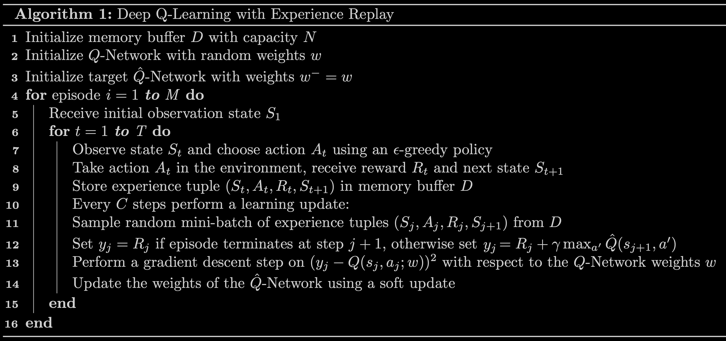

  
  Fig 4. Deep Q-Learning with Experience Replay.
  

  Credits

  A huge thank you to Professor Andrew Ng, whose Stanford Online course - Unsupervised ML: Recommenders and Reinforcement Learning - introduced me to this project, and for the guidance he provided throughout this project.