2017-IIIT-Summer-School-Machine-Learning.md

20170710

C. V. Jawahar - Intro to Deep Learning and Optimization (09:30 to 11:00)

• SVM

• Gradient Descent

• In addition to minimizing the reconstruction loss, we also want our model to be as simple as possible - so the magnitude of the weights must also be lesser

• PEGASOS: Primal Estimated sub-GrAdient SOlver for SVM

• Perceptron Learning: Perceptrons can only solve linearly-separable problems

• Deeper networks: MLP

• Backpropagation

Motivations for Deep Architecture

- Insufficient depth can hurt
- Brain seems to to deep

• Learning representations, automating this

• History: Fukushima (1980), LeNet (1998), Many-layered MLP with BackProp (tried, but without much success and with vanishing gradients), Relatively recent work

ALEXNET, Krizhevskky et al, 2012

- Winner of ImageNet 2012
- Trained over 1.2M images using SGD with regularization
- Deep architecture (60M parameters)
- Optimized GPU implementation (cuda-convnet)

Vineeth Balasubramanian - Backprop and Gradient Descent (11:30 to 13:00)

• Loss function from $J$ and $W_{i, j}$

• Backprop

• Gradient Descent

• Unfortunately backprop doesn’t work very well with many layers

• 40s: perceptrons; 50s: MLPs, apparently MLPs can solve any problem; 70s: MLPs cannot solve non-linear problems, like XOR; 90s: Hinton revived NN using non-linear activations and backprop

Local minima

- NN loss functions are non-convex
    - non-linear activations
    - NNs have multiple local minima
- So, weight initialization determines which local minimum your deep learning-optimized weights fall into
    - Also, weights are much more higher-dimensional
- Gradient descent: drop a blind person on the Himalayas, ask them to find the lowest point
- Non-identifiability problem/symmetry problem: any initialization is fine, any local minimum is OK
- “Almost all local minima are global minima”

Saddle Points

- Gradient=0 could also occur at saddle points!
- Saddle Point = minimum in one dimension, maximum in another
- As the number of dimensions increases, the occurrence of saddle points is also greater

• There is a community that does not believe in deep learning, because deep learning does not provide any guarantees. SVMs, etc. provide guarantees on finding an optimal solution. Such guarantees do not exist with deep learning

Cliffs

- Highly non-linear error surfaces may also have cliffs
- Occur for RNNs

Vanishing/Exploding gradient

- Gradients cascaded back might not have enough value by the first layers to change them much
- This is why we don’t want networks with too many layers: ResNet-1000 performed worse than ResNet-152
- Just to solve this problem in RNNs, LSTMs were invented
- Exploding gradients occur when gradients (maybe for activations other than sigmoid), are >1
- Exploding gradients could potentially be taken care of by clipping gradients at a max value

• Slow Convergence - no guarantee that:

  • network will converge to a GOOD solution
  • convergence will be swift
  • convergence will occur at all

• Ill conditioning: High condition number (ratio of max Eigenvalue to min Eigenvalue)

  • If the condition number is high, surface is more elliptical
  • If condition number is low, surface is more spherical, which is nice for descending

• Inexact gradients, how to choose hyperparameters, etc.

Batch GD, Stochastic GD, Mini-Batch SGD

• Batch GD: Compute the gradients for the entire training set, update the parameters

  • Not recommended, because slow

• Stochastic GD: Compute the gradients for 1 training example drawn randomly, update the parameters

  • Loss computed in Batch GD is the average of all losses from training examples
  • So Batch GD and SGD don’t converge to the same point
  • It’s not called Instance GD, it’s called Stochastic GD because the samples are drawn randomly. There are proofs of convergence given depending on the fact that samples are random.

• Mini-Batch SGD: Compute the gradients for a mini-batch of training examples drawn randomly, update the parameters

Advantages of SGD over Batch GD

- Usually much faster than Batch GD
- Noise can help! There are examples where SGD produced better results than Batch GD

Disadvantage of SGD

- Can lead to no convergence! Can be controlled using learning rate though

FIRST-ORDER OPTIMIZATION METHODS

Momentum

- Momentum == Previous Gradient
- Can increase speed when the cost surface is highly non-spherical
- Damps step sizes along directions of high curvature, yielding a larger effective learning rate along directions of low curvature
- Can help in escaping saddle points… But usually need second order methods to escape saddles

Accelerated Momentum

Nesterov Momentum

- Compute the Gradient Delta from loss at the weights updated by the previous gradient delta, then combine this Gradient Delta with the previous gradient delta
- Somehow works better than just momentum

Vineeth Balasubramanian - Backprop and Gradient Descent (13:30 to 15:30)

• There is an optimal learning rate with which one can reach the global minimum in one step. It is equal to the inverse of the double derivative at the point from which we start

RMSprop

AdaGrad

• Gradients diminish faster here… RMSprop takes care of this

Adam

- Similar to RMSprop with momentum

AdaDelta

• Works well in some settings

• Vanilla SGD may get stuck at saddle points

• Many papers use vanilla SGD without momentum, but best bet is Adam

• 

SECOND-ORDER OPTIMIZATION METHODS

• Gradient descent comes from approximating the Taylor series expansion to just the first order term

• By considering the second-order terms:

$${\delta}w = -\frac{f’(x_{0}}{f’’(x_{0})}$$

• So we see that the gradient update is inversely proportional to the second derivative!

• So, gradient update = $-H^{-1} * g$, where $H$ is the Hessian, $g$ is the gradient

• The ideal learning rates are the Eigenvalues of the Hessian matrix

• But, the Hessian is not feasible to compute at every step, let alone its inverse and eigenvalues

  • Computational burden
  • Cost-performance tradeoff is not attractive
  • There are some Newton’s methods to try, but they are attracted towards saddle points

• So we use other approximations like the Quasi-Newton methods

  • We compute one Hessian, then we compute the difference to add to get the next Hessian
  • E.g. LGFBS
  • Approximations: Fischer Information, Diagonal approximation

Conjugate Gradient Descent

- Two vectors $x$ and $y$ are said to be conjugate w.r.t. A matrix A if $x^{T}Ay = 0$
    - Here, y was the previous gradient update, A is the current Hessian, x is the new gradient update
- Compute the gradient, subtract some part of the previous gradient to get the conjugate component, compute the learning rate

Hessian-free Optimization

- Approximate the Hessian using the gradients

Natural Gradient

- Instead of using Euclidean distance to traverse along the error surface, travel along the surface of the manifold itself, the geodesic, the natural gradient
- [Revisiting natural gradients for deep networks, Razvan, ICLR 2014](https://arxiv.org/abs/1301.3584)

• Generally, second-order methods are computationally intensive, first-order methods work just fine!

RECENT ADVANCES

Gradient Descent

• Trying to understand the error surfaces, escaping saddles, convergence of gradient-based methods

• Deep Learning without Poor Local Minima, NIPS 2016

  • Theoretically showed that converging to a local minimum is as good as global minimum

• Entropy-SGD: Biasing Gradient Descent into Wide Valleys, ICLR 2017

  • Try to push gradient descent towards flat minima, because it is those minima into which most networks now converge to anyway

Escaping Saddle Points

• Escaping from Saddle Points, COLT 2015

  • Add Gaussian noise to gradients before update

• Degenerate Saddles

  • We found that most networks actually converge to saddles, not even flat minima
  • Saddles may be good enough

REGULARIZATION

• Difference between ML and Optimization is, ML tries to generalize, by designing an optimization problem first

• Theoretical ML: Empirical Risk Minimization (ERM). But, ERL can lead to overfitting

• Avoiding overfitting is Regularization

• It’s not important to get 0 training error, it’s more important to find the underlying general rule

Early Stopping

- Stop at an earlier iteration before training error goes to 0
- Of course not a very good idea
- Error-change criterion: if error hasn’t changed much within n epochs, stop
- Weight-change criterion: if change in max pair-wise weight difference hasn’t changed much, stop
    - Use max, it might be that only one direction is learning while all others are not

Weight Decay

- In addition to prediction loss, also add a loss with the magnitude (2-norm) of the weights
- Don’t give me a very complicated network
- Using L1-norm weight decay gives sparse solutions, meaning many weights go to 0, which helps in compression

DropOut

- Does model averaging
- In training phase: randomly drop a set of nodes in hidden layer, with probability p
- In test phase: use all activations, but multiply them with p
    - This is equivalent to taking the geometric mean of all the models if you ran them separately
- This is equivalent to using an ensemble
- Dropping nodes helps nodes in not getting specialized
- [Srivastava et al., JMLR 2014](http://www.jmlr.org/papers/volume15/srivastava14a.old/source/srivastava14a.pdf)

Regularization through Gradient Noise

- Simple idea: add noise to gradient
- [Neelakantan et al., Adding gradient noise improves learning for very deep networks, 2015](https://arxiv.org/abs/1511.06807)

DATA MANIPULATION METHODS

Shuffling inputs

- [Efficient backprop, LeCun](http://yann.lecun.com/exdb/publis/pdf/lecun-98b.pdf)

Curriculum Learning [Bengio et al., ICML 2009]

- Old idea, proposed by Elman in 1993
- Use simpler training examples first

Data Augmentation

- Data jittering, rotations, color changes, noise injection, mirroring
- [Deep image: Scaling up image recognition [Wu et al., 2015]](https://arxiv.org/abs/1501.02876)

Data Transformation

- Normalize/standardize the inputs to have 0 mean and 1 variance (refer to [Efficient Backprop paper](http://yann.lecun.com/exdb/publis/pdf/lecun-98b.pdf))
- Decorrelate the inputs (probably using PCA)

Batch Normalization

- DropOut fell out of favour after this was introduced
- Introduced Internal Covariance Shift
- Normalize the activation of a neuron across its activations for the whole mini-batch; then multiply with a variance and add a shift, and learn those mean and variance parameters in training
- BatchNorm eliminated the need for good weight initialization
- Also helps in regularization, by manipulating parameters with the statistics of the mini-batch

ACTIVATION FUNCTIONS

• Sigmoid: Historically awesome, but gradients fall to 0 if activations fall beyond a small range

• tanh: Same problem

• ReLU: created to counter the zero-gradient problem

  • But, ReLU is not differentiable
  • So we assume ReLU’s gradient as a sub-gradient: we define the gradient at 0
  • Dying ReLU problem: If even once the activation goes to negative, the ReLU does not let any neuron before it learn anything during backprop

• LeakyReLU: created to counter the Dying ReLU Problem

• Parametric ReLU: Same as LeakyReLU, but a different slope for negative values than LeakyReLU

• ELU

  • ReLU gives a positive value as the average, but they said the average is supposed to be 0
  • So they made ELU which maintains the average 0
  • For negative activations: ${\alpha}*({\exp}^{r} - 1)$

• MaxOut: generalization of ReLU

  • Take the max of a bunch of network activations

• ELUs are slowly becoming popular

• Never use sigmoid

• Try tanh, but expect it to work worse than ReLU/MaxOut

LABELS

• Try smooth labels (0.9 instead of 1)

LOSS FUNCTIONS

• Cross-entropy (will simplify to similar to MSE)

• Negative Log-Likelihood (will simplify to similar to CE)

• Classification Losses, Regression Losses, Similarity Losses

WEIGHT INITIALIZATION

• Don’t initialize with 0, no backpropagation, no learning

• Don’t initialize completely randomly, non-homogeneous networks are bad

• Most recommended: Xavier Init [Xavier Glorot, and Yoshua Bengio, Understanding the difficulty of training deep networks, AISTATS 2010]

  • Uses fan_in + fan_out info to draw samples from a uniform distribution

• Caffe made a simpler implementation

• He made a better implementation because Caffe’s didn’t work for ReLU: Delving deep into rectifiers, [He et al.]

20170711

Girish Varma - RNNs (09:30 to 10:30)

• RNNs

• Backpropagation through time

• Vanishing gradient problem

GRUs


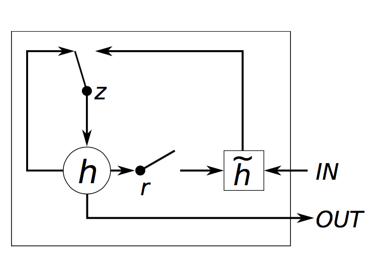
• Use tanh instead of sigmoid

• Has two gates: an Update Gate, and a Reset Gate

• Update Gate:

$$z_{t} = {\sigma}(W^{(z)}x_{t} + U^{(z)}h_{t-1})$$

• Reset Gate:

$$r_{t} = {\sigma}(W^{(r)}x_{t} + U^{(r)}h_{t-1})$$

• New memory content, as a combination of new input and a fraction of old memory:

$$hh_{t} = tanh(Wx_{t} + r .* Uh_{t-1})$$

• Updated memory content, as a combination of fraction of old memory content and complementary new memory content:

$$h_{t} = z_{t} .* h_{t-1} + (1 - z_{t}) .* hh_{t}$$

• We can see that if z_{t} is close to 1, we can retain older information for longer, and avoid vanishing gradient.

LSTMs

• LSTMs have 3 gates - Forget Gate, Input Gate, and Output Gate


Bi-directional RNNs

Stacking RNNs

Ankush Gupta (Oxford) - More on RNNs (11:00 to 12:30)

• Many flavours of Sequence-to-Sequence problems

• One-to-one (image classification), one-to-many (image captioning), many-to-one (video classification), asynchronous many-to-many (language translation), synchronous many-to-many (video labelling)

RNN

• [input, previous hidden state] -> hidden state -> output

• RNNs model the joint probability over the sequences as a product of one-step-conditionals (via Chain Rule)

• Each RNN output models the one-step conditional $p(y_{t+1} | y_{1}, … , y_{t})$

ENCODER-DECODER FRAMEWORK

• Sutskever et al., 2014; Cho et al., 2014

• Can stack RNNs together, but in my experience any more than 2 is unnecessary

• Thang Luong’s Stanford CS224d lecture

• Loss function: Softmax + Cross-Entropy

• Objective is to maximize the joint probability, or minimize the negative log probability

• The encoder is usually initialized to zero

• If a long sequence is split across batches, the states are retained

Scheduled Sampling

• During testing, it might just happen that the RNN gives one wrong output, and the error is compounded with time since the wrong output is fed as the next input!

• Scheduled Sampling is employed to take care of this

• During training, from time to time, sample from the output of the RNN itself and feed that to the next decoder input instead of the correct input

REPRESENTATION: Feature Embeddings / One-Hot Encoding

Domain-specific features

- ConvNet fc feature vectors for images
- Word2Vec features for words
- MFCC features for audio / speech
- PHOC for OCR (image -> text string)

One-hot encoding

Word-level

- Usually a large lexicon of ~100k words
- Cumbersome to handle
- Softmax is unstable to train with such huge fan out number

• So we go for:

Character-level

- Represent as sequence of characters

INFERENCE

• We don’t take argmax of the output probabilities because we will not optimize the joint probability then.

• Exact inference is intractable, since exponential number of paths with sequence length

• Why can’t we use Viterbi Decoder as in HMMs?***

Beam Search with Approximate Inference

• So, we compromise with an Approximate Inference:
  • We do a Beam Search through the top-k output classes per iteration (k is usually ~20)
  • So, we start with the token -> take the top-k output classes -> use each of them as the next input -> get the output class scores for each of the k potential sub-sequences -> sum the scores and take the top-k output classes -> use each of them as the next input …

LANGUAGE MODELLING

• Use RNN so as to capture context

SAMPLING/GENERATION

• Use “tau” as temperature to modify the output probabilities: s = s/tau
  • tau = 0 => prob is infinity for one word
  • tau = infinity => prob is flat, so you might not have trained your RNN at all

WHAT HAS RNN LEARNT?

• Interpretable Cells
  • Quote-detection cell: one value of the hidden state is 0 when the ongoing sentence is within quotes, 0 else
  • Line length tracking cell: gets warmer with length of line
  • If statement cell
  • Quote/comment cell
  • Code depth cell (indentation)

Ankush Gupta (Oxford) - More on RNNs (13:30 to 15:00)

ATTENTION MECHANISM

• Compare source and target hidden states

• Score the comparison between the hidden states of a source and a target node -> Do this for all encoder nodes with one target node (Make scores) -> Scale them and normalize w.r.t. Each other (Make Alignment Weights) -> Weighted Average

• Bahdanau at al., 2015 (attention mechanism)

  • Example of a well-written paper

Text Image to Text String (OCR)

- Recurrent Encoder-Decoder with Attention
- Fully convolutional CNN -> Bi-directional LSTM (to capture context) -> Attention over B-LSTM to decode characters

• Attention Mask: can tell which part of the input corresponded with maximal output

  • [Donahue et al., CVPR 2015]

• http://distill.pub/

CONCLUSION

• RNNs solve the problem of variable length input and output

• Solves knowledge of previous unit (by passing state)

• Can be trained end-to-end

• Finds alignment between input and outputs (through attention also)

Girish Varma - RNNs (14:00 to 15:00)

SCENE TEXT

• Use RNN to learn CRF

• Without character segmentation using RNN (Zisserman)

• https://arxiv.org/abs/1603.03101

  • Scene text with char-level language modelling
  • With attention modelling

Connectionist Temporal Classification (CTC)

• Removes need for chal-level segmentation

• Classifies simpl**e as simple

• CTC Loss

  • Let B be the decoding function: B(simple) = simple
  • p(simple) = {\sum}_{w that decodes to simple}p(w)
  • Loss = 1 - p(simple)

• But there are too many words that can decode to a simple word

• CTC with Dynamic Programming

• CNN + RNN + CTC: CRNN

HARD ATTENTION MODELLING

• Recurrent models of visual attention

• How to predict the window containing the next character? (in MNIST, say)

20170712

Sujit Gujar, IIIT Hyderabad - Introduction to Game Theory (09:00 to 10:30)

• Game Theory: mathematical model of conflict

• Elements: Players, States, Actions, Knowledge, Outcomes, Payoff or Utility

• Assumptions:

  • Players are rational beings trying to maximize their payoff
  • All players have complete information of the game

• Pure Strategy: deterministic steps

• Prisoner’s Dilemma:

	No Confess NC	Confess C
No Confess NC	-2, -2	-10, -1
Confess C	-1, -10	-5, -5

• Equilibrium: No player has any advantage deviating from it

• Playing (C, C) in the above Prisoner’s dilemma game is equilibrium.

• Some games have no equilibrium. Eg. Matching coins game:

	H	T
H	10, -10	-10, 10
T	-10, 10	10, -10

- In this case, players have to mix their strategies (of drawing H or T)

• Mixed strategy:

  • Playing actions (a_1, … , a_n) with probabilities (p_1, … , p_n)
  • Now, payoffs are not fixed, because strategies are randomized. We can only find Expected Payoff.
  • Mixed Strategy leads to Utility Theory by Neumann and Morgenstern

• In a Zero-Sum game, players follow a Min-Max Strategy

• GANs: Zero-Sum or Stackelberg Games

Vinay Namboodiri, IIT Kanpur - GANs - I (11:00 to 12:30)

• Problem to solve: unsupervised learning of (visual) representations

• Given access to a lot of data, we want to generate the data. Generation => We have understood the data.

• Initially, we wanted to learn some properties of data by trying to reconstruct the data using a deep network

  • Unlabelled Data -> Deep Network -> SGD Objective with Reconstruction Loss
  • But, this network simply formed the identity function w.r.t. the input data.
  • Didn’t at all work for data other than input data
  • Deep learning is a bad student who just memorises whatever is given to him, but doesn’t understand anything about the data

• Then, Hinton & Salakhutdinov, in Science 2006 made an autoencoder, where they put a bottleneck in the middle of the deep network

  • This worked well, the network learnt a compressed version of the input data
  • But it wasn’t there yet, it just learnt a fancy compression

• Denoising Autoencoders [Vincent et a;., ICML 2008]

  • Give purposefully corrupted data -> Autoencoder -> Reconstruct the original image without noise

• Sparse Autoencoder: Building High-level Features Using Large Scale Unsupervised Learning, ICML 2012

  • Used 16000 processors, 1 billion connections, 10M images to solve the problem of unsupervised learning once and for all
  • Worked mostly for cat videos. Google argued that that’s because YouTube is full of cat videos

• GANs work! How do we know? After all, Stacked Autoencoders also went only so far... Results!

  • BEGAN: Boundary Equilibrium GAN: Uses WGAN + encoders

• GANs: Counterfeit game analogy

• GAN Architecture Ian Goodfellow et al., 2014

  • z is some random noise = a latent representation of the images
  • GAN is not trying to reconstruct the input data
  • GAN is trying to make a model such that it generates data that is indistinguishable from real data
  • Generator vs Discriminator
  • G and D must be trained with complementary backprop gradients

• GAN Tutorial, NIPS 2016

• G tries to:

  • Maximise D(G(z)), or minimise (1 - D(G(z)))
  • Minimise D(x)
  • => Minimise D(x) + (1 - D(G(z)))

• D tries to:

  • Maximise D(x)
  • Minimise D(G(z)), or maximise (1 - D(G(z)))
  • => Maximise D(x) + (1 - D(G(z)))

• Thus, GAN objective function:

$$min_G max_D [D(x) + (1 - D(G(z)))]$$

• To analyze average behaviour, we take expectation: $$ min_G max_D E[D(x)] + E[(1 - D(G(z)))]

• At equilibrium, G is able to generate real images, and D is thoroughly confused

• Minimax Game:

$$ J^{(D)} = - {\frac{1}{2}}E_{x~p_{data}} log D(x) - {\frac{1}{2}}E_{z} log (1 - D(G(z)) $$ $$ J^{(G)} = - {\frac{1}{2}}E_{z} log D(G(z) $$

• But Goodfellow’s paper didn’t have good enough results… Next good progress was using DCGANs

• Unsupervised Representation Learning with DCGAN, Radford et al., ICLR 2016

  • Used a Deep Deconvolutional Network as the generator: Removed fc layers, changed activations, used BatchNorm
  • First realistic generation of images. Autoencoder, etc. produced blurry and erroneous images, this one made good sharp images
  • Also, latent vectors capture semantics as well, like - + =

• GAN Hacks by Soumith Chintala

• Data-dependent initialization; GitHub: magic_init

  • To change pre-trained weights according to new data format (-1 to 1 instead of 0 to 1, etc.)

Applications:

• Image from Text

• 3D Shape Modelling using GANs

• Image Translation: Pix2Pix

  • But this uses pairs of images

• CycleGAN

  • Trains from 1 to generated 2, and back from 2 to 1 (hence, cycle)

• Next Video Frame Prediction [Lotter et al., 2016]

Vinay Namboodiri, IIT Kanpur - GANs - II (13:30 to 14:30)

Unrolled GANs

• Based on letting the generator “peek ahead” at how the discriminator would see

• Does much better than DCGANs

STABILITY/CONVERGENCE PROBLEMS

Wasserstein GAN, GitHub

• Handles stability/convergence problems by letting the generator look ahead better

• Uses Earth-mover’s Distance / Wasserstein Distance

• But this means gradients could explode, so Weight Clamping is to be used (not BCE)

Improved WGAN (just 2 months later)

• Improved resilience against exploding gradients: Gradient penalty if it deviates from unit norm

INTERPRETABILITY PROBLEMS

InfoGAN

• Motivation: GANs use z in an entangled way; if a representation is unentangled, it could be made more interpretable

• Maximises Mutual Information

• Variational Maximisation of Mutual Information

  • Use an approximate function Q(C | X) for p(C=c | X=x)

• Sharing the net between Q(C | X) and the discriminator D(x)

• MNIST example with 10-dimensional discrete class, and 2 continuous classes (possibly width adn rotation)

• Faces example: pose, lighting, elevation

MODE COLLAPSE

Mode Regularized GAN [Che et al., 2016]

1. Metric Regularizer

   • Trying to learn an autoencoder

2. Mode Regularizer

MULTI-AGENT FRAMEWORKS

Generative Multi-Adversary Network [ICLR 2017]

• Multiple discriminators

• Formidable Adversary: hold up against all discriminators

  • Can be thought of as boosting
  • Generator could give up when the adversaries get too formidable

• Forgiving Teacher: have a variety of soft discriminators that can combine the outputs of multiple discriminators

MAD GAN (Multi-Agent Diverse Generation)

SEQUENTIAL GANs

Contextual RNN GAN for Abstract Reasoning Diagram Generation [AAAI 2017]

20170713

Kaushik Mitra, IIT Madras - Variational Inference and Autoencoders (09:00 to 10:30)

AUTOENCODERS

• Linear AE is same as PCA

• But fails:

  • Just memorizes the data, doesn’t understand the data
  • Overcomplete case: hidden dimension h has higher dimensions
  • Problem: identity mapping

• Sparsity as a regularizer

• De-noising autoencoder [Vincent et al.]

• Contractive Autoencoder

  • Learns tangent space of manifold
  • Minimize Reconstruction error + Analytic Contractive loss
  • Tries to model major variation in the data

• Can we generate samples from manifold?

  • We need the lower-dimensional distribution
  • Let’s assume it is Gaussian

VARIATIONAL AUTOENCODER

• Decoder samples z from a latent space, and decodes into the mean and variance from which to sample an x

• Encode: x -> Encode to a mean and variance for z, Decode: Sample a z -> Decode to a mean and variance for each dimensional value of x

• Terms:

  • Posterior: $p(z | x)$
  • Likelihood: $p(x | z)$
  • Prior: $p(z)$
  • Marginal: ${\int}p(x, z) dz$

• But, the marginal is intractable, because z is too large a space to integrate over

• So, decoder distribution p(x | z) should be maximized over q(z | x): minimize the log likelihood $E_{q(z | x)}[log p(x | z)]$

• Also, q(z | x) should be close to the z prior p(z) (Gaussian): minimize the KL Divergence $KL[q(z | x) || p(z)]$

• Importance Sampling

  • But, intractable

• Jensen’s inequality

** Concave: Graph is above the chord

• Variational Inference
  • Variational lower bound for approximating marginal likelihood
  • Integration is now optimization: Reconstruction loss + Penalty

Vineeth Balasubramanian - VAE (11:00 to 12:30)

VARIATIONAL AUTO-ENCODER

• Latent variable mapping [Aaron Courville, Deep Learning Summer School 2015]

  • Trying to discover the manifold in the higher-dimensional space, trying to find the lower-dimensional numbers

• Example of Face Pose in x axis and Expression in y axis from the Frey Face dataset

• We can sample from z and generate an x using a transformation G: x = G(z)

• How to get z, given the x’s in our dataset

• [Auto-Encoding Variational Bayes, Kingma and Welling, ICLR 2014]

• Estimate ${\theta}$ without access to latent states

• PRIOR: Assume Prior $p_{\theta}(z)$ is a unit Gaussian

• CONDITIONAL: Assume $p_{\theta}(x | z)$ is a diagonal Gaussian, predict mean and variance with neural net

• So, from a sampled z, estimate a mean and variance from which to sample an x

• From Bayes’ theorem,

$$ p_{\theta}(z | x) = {\frac{p_{\theta}(x | z) * p_{\theta}(z)}{p_{]theta}(x)}} $$

• Here, p_{\theta}(x | z) can be found from the decoder network, p_{\theta}(z) is assumed to be a Gaussian, BUT $p_{]theta}(x)$ is intractable.

  • Because, to find $p_{]theta}(x)$, we need to integrate over all x’s on all values of z

• So, $p_{\theta}(z | x)$ is very hard to find, since we don’t know $p_{]theta}(x)$

• Instead, we approximate this posterior with a new posterior called $q_{\phi}(z | x)$, and then try to minimize the KL divergence between $q_{\phi}(z | x)$ and $p_{\theta}(z | x)

• We get $q_{\phi}(z | x)$ from the encoder network.

• Data point x -> Encoder: mean, (diagonal) covariance of $q_{\phi}(z | x)$ -> Sample $z$ from $q_{\phi}(z | x)$ -> Decoder: mean, (diagonal) covariance of $p_{\theta}(x | z)$ -> Sample $hat{x}$ from $p_{\theta}(z | x)$

• Reconstruction loss for $hat{x}$, Regularization loss on prior $p_{\theta}(x)

• Reparametrization trick

  • Because we’re sampling in between, it is not back-propagatable, since we need to differentiate through the sampling process

• Laurent Dinh Vincent Dumoulin’s presentation

Semi-Supervised VAEs

- M1 - vanilla VAE: use z to generate x
- M2 - use z and a class variable y to generate x
- M2 - use some inputs with labels and some without
- M1 + M2
    - shows dramatic improvement
- Conditional generation using M2

Conditional VAE

- z does not split the different classes, instead class label is given as a separate input

Importance-Weighted VAE, Salakhutdinov’s group, ICLR 2016

De-noising VAE

• Added noise to input

• Took $q_{\phi}$ as a mixture of Gaussians

Deep Convolutional Inverse Graphics Network

• Train by a subset of components of z with one type of variation
  • Vary lighting and only sample from a subset of components, etc.

Adversarial Autoencoders

• Ask a Discriminator to make out the difference between a sample z from the Encoder, and a sample from the actual prior (Gaussian)

Applications

- Image and video generation
- Super-resolution
- Forecasting from static images
- Inpainting

Vineeth Balasubramanian - VAE (13:30 to 14:30)

Recurrent VAE

Kaishuk Mitra, IIT Madras (14:30 - 15:30)

AUTOREGRESSIVE MODELS

RIDE by Theis et al.

• Recurrent Image Density Estimator

• Structure: SLSTM + MCGSM

• Spatial LSTM: Kind of a 2D LSTM

• Mixture of Conditional Gaussian Scale Mixtures

Pixel RNN by Oord et al.

• Improvisation over sLSTM

• Uses two different LSTM architectures: RowLSTM, Diagonal BiLSTM

Pixel CNN

• Replace RNNs with CNNs

• Can’t see beyond a point, but much faster to train

Conditional Pixel CNN

PixelCNN++

• PixelCNN produces discrete distribution, this one produces continuous distribution

DISCRIMINATIVE MODELS

• Image de-noising, image de-blurring, image super-resolution

• Con: there has to be a separate model each type of degradation

• Degraded image: Y = A*X + n

• Generative modelling: versatile and general

• MAP inference: arg max_X p(Y | X)*p(X)

• Traditional approach: Dictionary learning

  • Video dictionary [Hitomi et al., 2011]
  • But, difficult to capture long-range dependencies

• GANs are out of the question, since they don’t model p(x) explicitly. MAP inference is not possible.

• VAE takes a lot of computation: they approximate p(x) with a lower bound

20170714

Ravindran Balaraman, IIT Madras - Deep RL - I (09:00 to 12:00)

• Sutton and Barto’s book

• RL examples

• Arcade Games [Mnih et al., Nature 2015]

  • Learn to play from the video, from scratch

• Mastering the game of Go [Silver et al., 2016]

• Alpha Go [Silver et al., Nature 2016]

THEORY

Markov Decision Process

- MDP: M is the tuple: $<S, A, {\Phi}, P, R>$
- $S$: set of states
- $A$: set of actions
- ${\Phi} \subseteq SxA$: set of admissible state-action pairs
- $P: {\Phi}xS -> {0, 1}$: probability of transition
- $R: {\Phi}xR$: expected reward
- Policy: ${\pi}: S->A$ (can be stochastic)
- Maximize total expected reward
- Learn an optimal policy

• Checkerboard/grid, with some squares blacked out, need to reach a corner (Goal) from one corner in the shortest possible path

  • Reward cannot be distance from goal, since that defeats the purpose of reinforcement learning
  • Reward can be -1 for every step taken

• Goal must be outside the agent’s direct control, thus outside the agent

• Agent must be able to measure success: explicitly, frequently during its lifespan

• We want to maximize the expected return, E[R_t]

• Continuous tasks: R_t = r_0 + r_1 + …

• Discounted tasks: R_t = r_{t+1} + {\gammma}r_{t+2} + {\gammma}^2t_{t+3} + …

  • {\gammma} -> 0 => short-sighted, {\gammma}->1 => far-sighted

• Value function: Expectation of total return

• Bellman Equation for policy {\pi}:

$$ R_t = r_{t+1} + {\gammma}r_{t+2} + {\gammma}^2r_{t+3} + … = r_{t+1} + {\gammma}R_{t+1} $$

So,

$$ V^{\pi}(s) = E_{\pi}[R_t | s_t = s] = E_{\pi}[r_{t+1} + {\gammma}V(s_{t+1}) | s_t = s] $$

Or,

$$ V^{\pi}(s) = {\sum}a {\pi}(s, a) {\sum}{s’} P^{a}{ss’}[R^a{ss’} + {\gammma}V^{\pi}(s’)] $$

• Using Action Value Q:

$Q^{\pi}(s, a)$ is the expected return from state s, given an action a. So,

$$ Q^{\pi}(s, a) = {\sum}{s’} P^{a}{ss’}[R^a_{ss’} + {\gammma}V^{\pi}(s’)] $$

So,

$$ V^{\pi}(s) = {\sum}_a {\pi}(s, a) Q^{\pi}(s, a) $$

• Optimal Value function: the estimated long-term reward that you would get starting from a state and behaving optimally

• Optimal Policy: a mapping from states to actions such that no other policy has a higher long-term reward

• Bellman Optimality Equation for V*:

The value of a state under an optimal policy must equal the expected return for the best action for that state.

$$ V*(s) = max_{a{\in}A(s)} {\sum}{s’} P^a{ss’}[R^a_{ss’} + {\gammma}V*(s’)] Q*(s) = max_{a{\in}A(s)} {\sum}{s’} P^a{ss’}[R^a_{ss’} + {\gammma}max_{a’}Q*(s’, a’)] $$

V* and Q* are the solutions to this system of non-linear equations.

• One-step Q-learning: $$ Q(s_t, a_t) <- Q(s_t, a_t) + {\alpha}[r_{t+1} + {\gammma}max_a Q(s_{t+1}, a) - Q(s_t, a_t)] $$

The alpha-term is called Temporal Difference error (TD Error).

• REINFORCE [Williams, 1992]

• Simple Monte-Carlo Policy Gradient Algorithm

• Policy Gradient Theorem

• Use a parameterized representation for value functions and models

Tejas Kulkarni, Google Deep Mind - Deep RL - I (12:00 to 14:00)

• Fundamentals, Value-based Deep RL, Policy-based Deep RL, Temporal Abstractions in Deep RL, Frontiers

• Reinforcement Learning: a sequential decision-making framework to express and produce goal-directed behaviour

• Deep Learning: a representation-learning framework to re-present, interpolate and sometimes extrapolate raw data at multiple levels of spatio-temporal abstractions

• Deep RL: Simultaneously learn representations and actions towards goal-directed behaviour

• We use Deep Learning, but extend the loss function temporally

• State = g(x_t) given observations x_t. Here, g(.) denotes a deep neural network

• Deep Q Network (DQN): Predict Q using a neural network

• ATARI: 84x84 screen, 18 discrete actions

• But, introducing a neural network made the problem divergent

  • So, make a copy of the network called Target Network, and update it every few episodes

• Also, game score ranges are not same across games

  • So, clip the scores at +1 and -1 for robust gradients.
  • But the system loses the ability to differentiate between arbitrary reward values!

• Experience Replay:

  • Sample correlations can cause divergence during optimization
  • Alleviate this issue by storing samples in a large circular buffer called Replay Buffer
  • Mnih et al., Human-level control through deep reinforcement learning

• Deep Successor Q Network Deep Successor Reinforcement Learning, Kulkarni, Saeedi, et al.

• Deep Actor-Critic Algorithms

• Variance reduction in Policy Gradients

• Asynchronous Advantage Actor-Critic (A3C)

• Adding Auxiliary Losses to A3C [Reinforcement Learning with unsupervised auxiliary tasks, Jaderberg et al.]

• Temporal Abstractions

  • [Options framework Sutton, Precup, and Singh, Between MDPs and semi-MDPs: A framework for temporal abstraction in reinforcement learning
  • Have deep values as well

• Hierarchical DQN

20170715

Mitesh Khapra, IIT Madras - Deep Learning for Word Embeddings

• “You shall know a word by the company it keeps” - Firth., J. R. 1957:11

• In One-Hot Encoding, every pair of points is sq(2) Euclidean distance between them. Using any distance metric, every pair of words is equally distant from each other. But we want an embedding that captures the inherent contextual similarity between words

• A Co-occurrence Matrix is a terms x terms matrix which captures the number of times a term appears in the context of another term

  • The context is defined as a window of k words around the terms
  • This is also called a word x content matrix

• Stop words will have high frequency in the Co-occurrence Matrix without offering anything in terms of context. Remove them.

• Instead of counts, use Point-wise Mutual Information:

  • PMI(w, c) = log(p(c | w)/p(c)) = log(count(w, c)*N/(count(c)*count(w)))
  • So Mutual Information is low when both words occur quite frequently in the corpus but don’t appear together very frequently
  • PMI = 0 is a problem. So, only consider Positive PMI (PPMI): PPMI=PMI when PMI>0, PPMI=0 else

• It’s still very high-dimensional and sparse. Use PCA:

  • SVD: X_{mxn} = U_{mxk}{\Sigma}{kxk}V^T{kxn}, where k is the rank of the matrix X
  • Make k = 1, or any number lesser than the rank of X, and U*{\Sigma}*V^T is still an mxn matrix, but it is an approximation of the original X, wherein the vectors are projected along the most important dimensions, and it is no longer sparse

• XX^T is the matrix of the cosine similarity between the words. XX^T(i, j) captures the similarity between the i^{th} and j^{th} words.

• But this is still high-dimensional. We want another approximation W, lesser dimensional than X, s.t. WW^T gives me the same score as XX^T

  • $XX^T = (U{\Sigma}V^T)(U{\Sigma}V^T)^T = (U{\Sigma}V^T){V{\Sigma}U^T} = U{\Sigma}(U{\Sigma})^T$, because V is orthonormal (V*V^T = I).
  • So, U{\Sigma} is a good matrix to be our W, since it is low-dimensional (m x k).

• Iti pre-deep learning methods

CONTINUOUS BAG OF WORDS (CBoW)

• Given a bag of n context words as the input to a neural network, predict the (n+1)^{th}word as the softmax output of the network.

Girish Varma, IIIT Hyderabad - Model Compression (11:10 to 12:30)

• Reduce memory usage by:

  • Compressing matrices: using sparse matrices, quantization
  • Design architecture to have lesser memory

• Pruning:

  • Fine pruning: prune the weights
  • Coarse pruning: prune neurons and layers
  • Static pruning: pruning after training
  • Dynamic pruning: pruning during training

WEIGHTS

Weight Pruning

• Drop the weights below a threshold

• Can be stored in an optimized way of matrix is sparse

• Ensuring sparsity: use L1 regularizer

  • L1 (absolute value) regularizer has more slope near 0 than L2 (quadratic) regularizer, so it is more likely to push values to 0 than L2

• DeepNeuron: Simplifying the Structure of Deep Neural Networks [Wei Pan, Hao Dong, Yike Guo]

  • Regularize the weights, drop neurons with weights close to 0

• Learning Neural Network Architectures using Backpropagation [Suraj Srinivas, R. Venkatesh Babu]

Quantization

• Compressing Deep Convolutional Neural Networks using Vector Quantization, Lubomir Bourdev

  • Binary quantization leads to 20% drop in top-5 accuracy in ILSVC
  • Reisdual quantization

• Deep Compression: Compressing Deep Neural Networks with Pruning, Trained Quantization and Huffman Coding, Song Han et al.

  • Non-uniform weight quantization via k-means clustering
  • Pruning + Quantization
  • Won best paper award in ICLR 2016

• XNOR-Net: Image Classification using Binary Convolutional Neural Networks, Ali Farhadi

  • Really fast
  • Uses fixed-point representation

ARCHITECTURE

• What about architectures with compressed representations?

GoogLeNet

• First architecture with improved utilization of computing resources

• Inspired from Network in Network

• Used a cascading of Inception modules

• Used Global Average Pooling as a replacement for fc layers

  • 90% of parameters in AlexNet and VGG Net were in fc layers

  • fc layers were prone to overfitting
  • Global Average Pooling pools an entire filter channel into 1 average value. So last conv layer needs to have as many channels as the number of output classes

Inception v2

• Remove 5x5 convolutions; instead, use only 1x1 and 3x3, and use 2 3x3 to replace the 5x5 convolution

  • This itself produced 28% reduction in size

• Spatial factorizing into asymmetric convolutions

Xception

- Similar to inception; in the inception module, has a common 1x1 convolution and then apply 3x3 convolutions on top.

SqueezeNet

- Applies all the compression techniques

Mobile Nets

- More depth-wise convolutions

Student-Teacher Networks

• Do deep networks really need to be deep?

• Distilling the knowledge in a neural network, Hinton, NIPS-W 2014

• Train a smaller network (student) with the hidden outputs of a deeper network (teacher)!

  • MIMIC Model (Multiple Indicator, Multiple Cause)

• Teacher could have resolved errors in labels

FitNets, Bengio

- Try to minimize error between student and teacher at intermediate states as well!

Fast Algorithms for Convolutional Neural Networks, Andrew Lavin, Scott Gray](https://arxiv.org/abs/1509.09308)

- Uses Winograd’s minimal filtering algorithms to reduce number of architecture ops