C. V. Jawahar - Intro & Background (09:30 to 11:00)
-
Obj: to understand and learn the recent-ish advances in the CV scene in the world
-
Last year summer school: basics of deep learning, touched CV; this year, 2 summer schools: one for CV; the other for Deep Learning (with some overlap)
-
Typical day plan: Breakfast, Session 1, Break, Session 2, Lunch, Session 3a, Session 3b, Break, Demo/La/Tutorial, Lab/Practice & Quiz, Dinner
-
CV Goal - To make computers understand images and videos
-
Scene classification (outdoor, lakeside...), Object Classification (is that a car, or...), Object Detection (where is the car, ...), Semantic Segmentation (in what all pixels is the car, ...), Pose Estimation (which direction is the car facing, ...)
-
Image -> Text: Image Annotation, Image Caption Generation, Image Description
-
History of CV - face detection, ...
-
Recognition: Classification (Instance recognition, Category recognition, Fine-grain classification), ... , Labels
-
Challenges : Occlusions, truncations, scale/size, articulation, Inter-class similarity, Intra-class variation
-
Variations in problems: Binary Classification, Multi-class, Multi-Label, Multi-output
-
Feature extraction: I -> X, Classification: X -> Y; End-to-end: can we do I -> Y?
-
Caltech 101 (2003): dataset for basic-level classification; objects from 101 classes; considered a toy dataset now; possibly gained high accuracies quickly because images were captured for the purpose of classification
-
PASCAL VOC (2005-2012): 20 object classes, 22,591 images; multiple tasks: Classification, Detection, Segmentation; van Gool, Zisserman, IJCV 2015
-
ImageNet (ILSVRC) (2010): 1000 object classes, 14,197,122 images; Classification as Top-5, Karpathy, Fei-Fei, IJCV 2015
-
COCO: harder than ImageNet; 80 object classes, 300,000 images; Describe Images, Human Keypoints
-
More datasets...
-
Classification evaluation: Overlapped area between true bounding box and predicted? Intersection? Intersection/Union?
-
Basic Detection: Image -> features of every possible rectangle -> rectangle with max probability of class; Update: region proposal
-
Evaluation metric: Average Precision (AP), Mean AP (Precision averaged over all thresholds of classification)
-
Success of classification/detection: ML, data, computation (GPUs)
- Extremely low-level vision: filtering
- Edges: Canny (1968), Sobel, Prewitt, ...
- Textures: Viola-Jones (2001), ...
- Histograms: [SIFT (Lowe, 1999)](https://www.robots.ox.ac.uk/~vgg/research/affine/det_eval_files/lowe_ijcv2004.pdf), Shape contexts (Malik, 2001), Spacial Pyramid Matching (Lazebnik, Schmid, Ponce, 2006)](http://www.vision.caltech.edu/Image_Datasets/Caltech101/cvpr06b_lana.pdf), [DPM based on HOG (Felzenswalb et al., 2010)](https://cs.brown.edu/~pff/papers/lsvm-pami.pdf)
- Bag of Words: histograms happened in Text domain, so we brought them to images, like histograms of textures
- Bag of Visual Words: histogram of predefined visual textures (Visual Words)
- [Bag of Words (Zisserman, 2003)](http://www.robots.ox.ac.uk/~vgg/publications/papers/sivic03.pdf), SIFT (Lowe, 1999, [2004]((https://www.robots.ox.ac.uk/~vgg/research/affine/det_eval_files/lowe_ijcv2004.pdf))), [HOG+SVM (Dalal and Triggs, 2005)](http://www.csd.uwo.ca/~olga/Courses/Fall2009/9840/Papers/DalalTriggsCVPR05.pdf)
- Semantic segmentation
- Deep Learning: you can learn low-level to mid-level to high-level features automatically without manual intervention
- One-Hot to Rich Representations: [word2vec](https://arxiv.org/abs/1301.3781) in text (Mikolov, 2013)
- CBOW: Given a sequence of words, can you predict the missing middle word? Skip-gram: Given one word, can you predict the sequence of words before and after?
- As Clustering: group similar pixels together (unsupervised), distance based on color and position; not really acceptable anymore for any decent segmentation
- K-Means, [Normalized Graph Cut](https://people.eecs.berkeley.edu/~malik/papers/SM-ncut.pdf) (Malik, 2006)
- Graph Cut: Label Pixels as Background (Source) or Object (Sink), make that as a graph, cut the graph so that there is no path between Source and Sink; use MRF, etc. for making and cutting the graph
- Graph Cut by Energy Minimization: pairwise constraint on pixel values
- [Grab Cut (Rother et al., 2004)](https://cvg.ethz.ch/teaching/cvl/2012/grabcut-siggraph04.pdf) using Iterated Graph Cuts: User initialization, iterate: learn foreground, learn background; user initialization provides supervision
- Superpixels: group pixels together, now apply same techniques by assigning labels to superpixels instead of pixels
- Semantic Segmentation: Class Segmentation (where are persons?), Instance Segmentation (class: persons, segment boundaries of each person), Segmentation from expression ("wearing blue")
C. V. Jawahar - Intro to DL for CV (11:30 to 12:45)
-
Linear Classifiers
-
Nearest neighbours
*Cholesky Decomposition
-
Nearest neighbours for image annotation: "A new baseline for image annotation"
-
SVM
- Max-margin classifier
- Key words: Training, testing, generalization, error, complexity (number of parameters), generative classifiers, discriminative classifiers
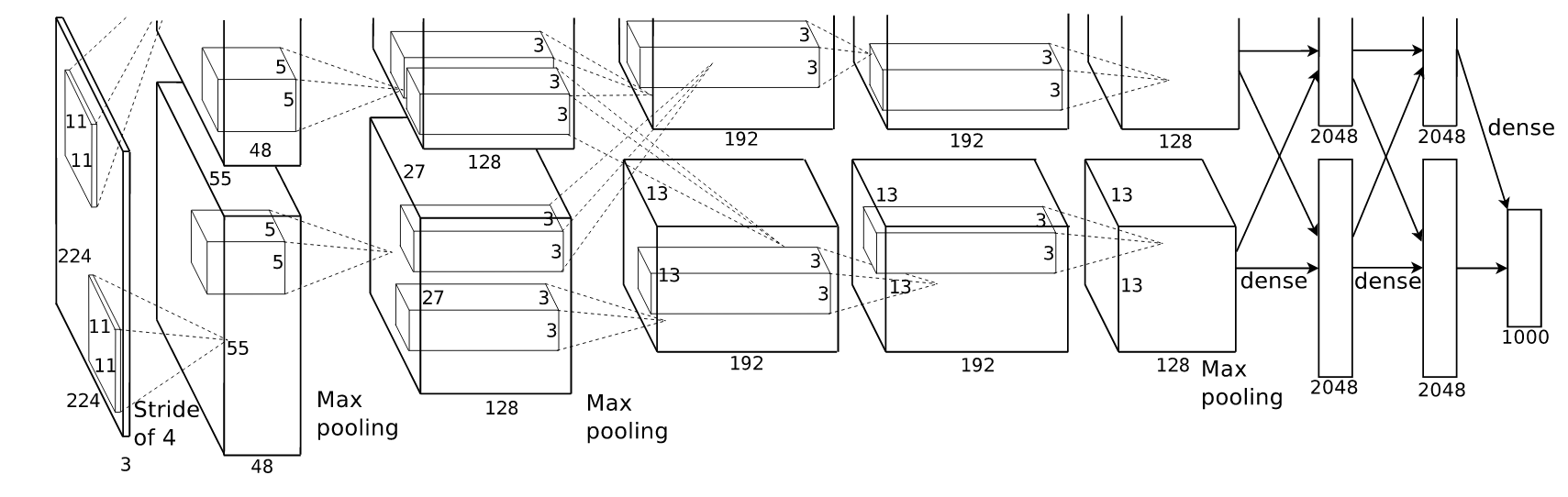
- After such classifiers came AlexNet which suddenly improved error from ~25% to ~15%
- Appreciate what Alex did, it was very difficult to do the first time
-
Over the years, deeper networks brought the ImageNet error rate down to human level
-
LeNet (1989) - LeNet (1998) - AlexNet (2012) comparison
-
MLP
-
Back-propagate through the networks using gradient descent
-
CNN: Locally connected networks with shared weights
- FC (too many weights/parameters) -> Locally connected filters (many many weights, one set per, say, 3x3 filter going over the original image) -(BIG JUMP)> use shared weights to convolve over an image (much lesser number of parameters) => Convolutional layer with 1 feature map -> Convolutional layer with multiple feature maps
- It is observed that the filters learned this way are similar to the filters we had manually tried to make many years ago
- Pool: Shrink the output size by choosing only some of the outputs
- Stride: Jump pixels to reduce number of parameters
-
Activation functions: Pass the output of the CNN through a non-linearity to generalize
-
Stack such layers together - ...=-ConvPoolNorm-ConvPoolNorm-...; this behaves similar to an MLP
-
This is what Alex did. “ImageNet Classification with Deep Convolutional Neural Networks”
-
CNN features are generic: Now, we can use the same network, remove the last classification layer, and use the features learnt till the penultimate layer to classify other object categories!
- Train the CNN on a very large dataset like ImageNet
- Reuse the CNN to solve smaller problems by removing the last (classification) layer
- Extend to more classes (eg. from 1000 classes to another new 100 classes)
- Extend to new tasks (eg. from object classification to scene classification) (Transfer Learning)
- Extend to new datasets (eg. from ImageNet to PASCAL)
- People tried to see why same features could be used for different tasks
- [“How transferable are features in deep neural networks?”, Bengio, NIPS 2014](https://arxiv.org/abs/1411.1792)
-
Other popular deep architectures: Autoencoder, RBM, RNN, …
-
Summary
Girish Verma - AlexNet and Beyond (13:30 to 15:30)
- AlexNet (ImageNet 2012 Winner)


- In each iteration, randomly choose some weights to zero out their outputs
- Train the network
- At testing time, use all neurons, don’t zero
- So, each neuron does not depend a lot on other neurons, we are eliminating such dependencies
- Obviously, it takes more number of epochs to achieve the same training accuracy as that without Dropout, but the testing accuracy increases very well
- Dropout was used in AlexNet
ZFNet (ImageNet 2013 Winner)

- Looks very similar to AlexNet, but they tried to interpret the feature activity in the intermediate layers
- They visualized the outputs of each layer
- ZFNet was an improvement on AlexNet by tweaking the architecture hyperparameters, in particular by expanding the size of the middle convolutional layers
- Also, they did Input Jittering
- #### Input Jittering
    - Scale down the largest dimension to 256
    - Consider 5 images as sub-images of this 256-sized image of 224x224 size
    - Flip the images to make a total of 10 images
    - Use all of these to train the network
- Winner of ImageNet localization task 2013
- Training to classify, locate and detect objects improves accuracy of all three
- No need to jitter, takes care of cropping and scaling within the network itself
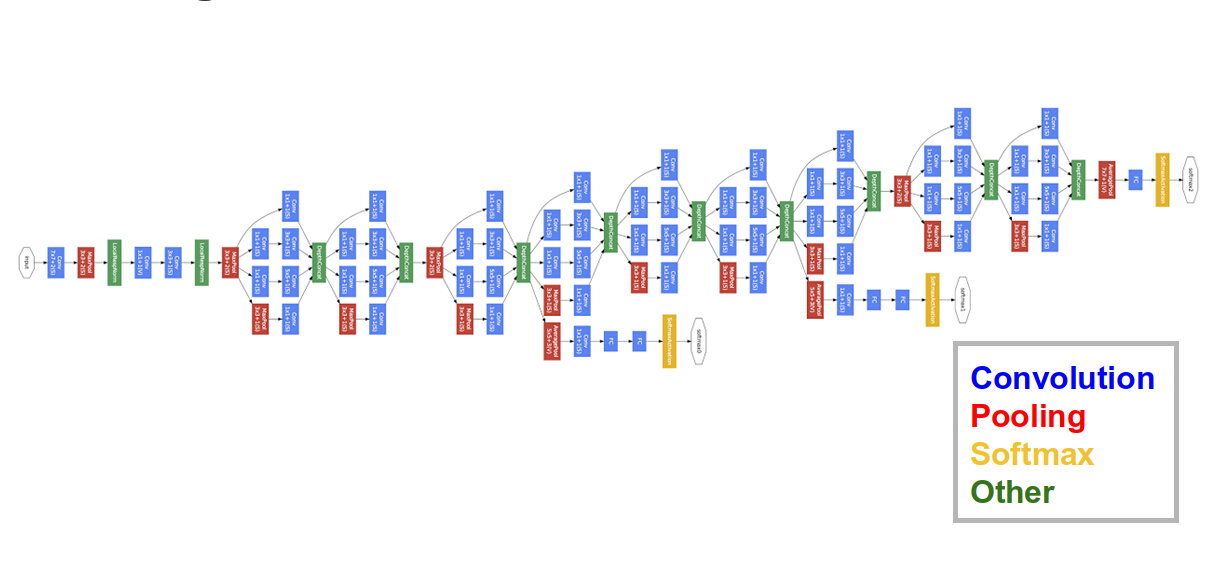
GoogLeNet/Inception (runner up in ImageNet 2014)

- They simply doubled the number of hidden layers to 22
- They saw that the FC layers contain the most number of parameters. So they reduced the number of parameters in the FC layer to the bare minimum, instead compensating via the convolutional layers
- They carefully designed convolutional layers called Inception modules
- #### Inception Modules

    - Each inception module is performing 1x1, 3x3, 5x5 and 3x3 with max pooling simultaneously
- Stack Inception modules together
VGGNet (winner of ImageNet 2014)
- Deeper is better philosophy: multiple 3x3 filter layers have the same effect as 5x5 or 7x7 or bigger filters
- Uses 19 layers
ResNet (winner of ImageNet 2015)

- Network which won the competition was 110 layers deep
- Deep networks have vanishing gradient problem. ResNet overcomes this using Skip connections
- Skip connections: simply add gradients from a much further layer with those from regular backprop
- Train multiple networks and take a majority vote
- Batch Normalization (from CS231n lecture slides)
- Classification: get the object label, Localization: get the bounding box of the object
- Use a classification network to classify the object
- Use another network to get the bounding box
- Task: put a bounding box on every instance of any class

- Image -> Extract Region Proposals -> Compute CNN features for each of the proposed region -> Classify regions
- But, many region proposals is a problem
- Operation can be optimized by passing full image through CNN, and then looking at the proposed region’s outputs from CNN
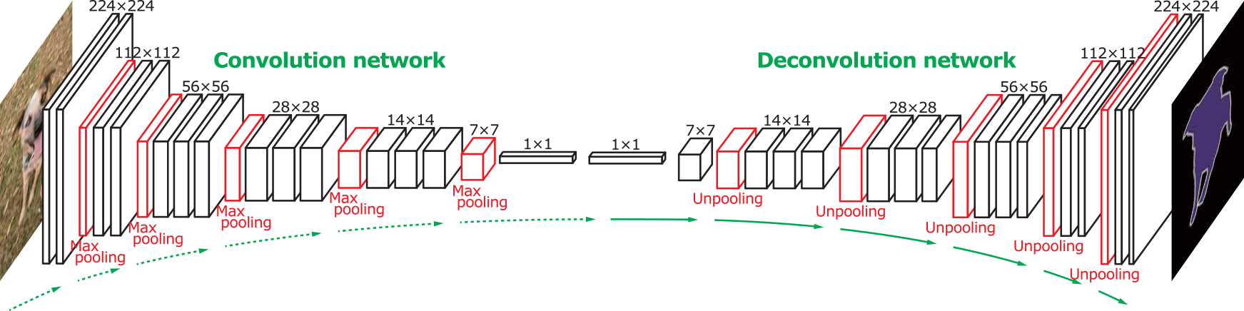
- We can make the output layer have same dimensions as input image, and value/third dimension with class label
- We need to unpool to get the same image size
- Used in [DeconvNet](http://arxiv.org/abs/1505.04366) we convolve and then deconvolve to get the same image size as the output size
 - Good link!
- Each instance of a class is labeled separately
- Convert x_1, x_2, … , x_s to o_1, o_2, … , o_t
- RNNs are designed to remember long-term dependencies
-
SceneText (OCR problem): RNN + CNN
-
Image and Video captioning - Venugopalan et al., “Sequence to Sequence - Video to Text”, 2015
-
- Pass image through CNN, question through RNN, then point-wise multiply the two outputs and pass through a fully-connected network
- Keras implementation
- Use PyTorch
- CNNs, ResNet
Chetan Arora (IIIT Delhi) - Detection (09:30 to 12:20)
-
Detection: Object Location, Object Attributes
-
Applications: Instance Recognition, Assistive Vision, Security/Surveillance, Activity Recognition (in videos)
-
Challenges: Illumination, occlusions, background clutter, intra-class variation
- Geometrical era
    - Fit model to a transformation between pairs of features
    - Machine Perception of Three Dimensional Solids, a PhD Thesis in 1963
    - It’s invariant to camera position, illumination, internal parameters
    - Invariant to similarity Tx of four points
    - But, intra-class variation is a big problem
- Appearance Models
    - Eigenfaces ([Turk and Pentland, 1991](http://www.face-rec.org/algorithms/PCA/jcn.pdf))
    - Other appearance manifolds
    - Requires global registration of patterns
    - Not even robust to translation, forget about occlusions, clutter, geometric Tx
- Sliding Window
    - Like, Haar wavelet by Viola Jones on a sliding window ([Viola and Jones, 2001](http://www.vision.caltech.edu/html-files/EE148-2005-Spring/pprs/viola04ijcv.pdf))
    - THE method until deep learning came, because it’s pretty fast
    - But, we need non-maximal suppression
- Local Features
    - SIFT (Lowe, 1999, 2004), SURF
    - Bag of Features: extract features -> bag them into words -> match stuff through words, not features
    - Spatial orientation is ignored
- Parts-Based Models
    - Model: object as a set of parts, noting relative locations between parts, appearance of each part
    - [Fischer and Elschlager, 1973](http://dl.acm.org/citation.cfm?id=1309318)
    - Constellation model: recognizing larger parts in objects
    - Discriminatively-trained PBM: eg. HoG ([Ramanan, PAMI 2009](https://cs.brown.edu/~pff/papers/lsvm-pami.pdf)); can recognize object even if whole object can’t be seen
- Present ideas: global+local features, context-based, deep learning
-
ImageNet: excellent competition for image classification
-
AlexNet (2012) won in 2012, changed the game
-
CNN: Local spatial information is transmitted through the layers; fine-level information in channels, location-level in neurons themselves
-
Convolutional layers are translation-invariant
-
Responses from the layers are composed: one layer fires when it sees a head, a shoulder, the next layers fires when it sees both, etc.
-
Convolutional layers can work with any image size, it’s just that the layers can be scaled accordingly
-
HoG by Convolutional Layers:
- HoG: Compute image gradients -> Bin gradients in 18 direction -> Compute cell histograms -> Normalize cell histograms
- CNN: Learn edge filters -> Apply directional filters + gating (non-linearity) -> Sum/Average Pool -> LRN
- So the same steps of HoG can be equivalently produced by a CNN, and even better because CNN can decide the bins, and other steps that were hitherto hand-engineered
-
HoG, Dense SIFT, and many other “hand-engineered” features are convolutional feature maps
-
Features in feature maps (one channel of any convolutional layer) can be back-tracked to a visual feature in the original image
-
What if we apply CNNs to object classification + localization?
-
We could slide a window on the original image, input each image into, say, AlexNet, and find the window with max firing of object, say cat
-
But Sliding Window approach in this case is computationally expensive, because too many windows (Viola-Jones, etc. are not computationally expensive)
-
- Using AlexNet, in addition to a last layer to predict the object class, use another last layer to predict the 4 numbers of a bounding box
- Total loss = Softmax loss of object class label + L2 loss of bounding box
-
But this fails when there are multiple objects, or multiple instances of the same object!
-
So let’s try to reduce the number of windows using Region Proposals
-
- Extract Region Proposals -> Resize each region to standard size -> Find Convolutional features -> Classify each region (maybe using SVM), and do linear regression for bounding box within proposed region
- Training for R-CNN is not very accurate at first, and it is very slow
- Ad-hoc training objectives (use an AlexNet pre-trained with ImageNet):
- Fine-tune network with softmax classifier (log loss)
- Train post-hoc linear SVMs (hinge loss)
- Train post-hoc bounding box regressing (least squares)
- But, this takes a looooong time to train, and a long time to infer (the class and bounding box)
-
- Instead of cropping the original image by the proposed regions and passing them through the network, pass the entire image, and then crop the extracted feature (say, at Conv5, the last convolutional layer in AlexNet) according to the region proposals!
- But the extracted cropped-ish feature (feature cropping is not advisable, features are different from images) is of variable size depending on the size of the proposed region
- So use Bag-of-Words and Spatial Pyramid Matching (SPM) to extract a uniform-sized vector at the end of the convolutional layers to input to the Dense layers
- SPM: Make grids with pyramidally increasing size, pool the features into the grids, use these grids as the input to the Dense layers
- This is what SPP Net [He et al., ECCV14] did
- So SPP Net fixes the inference speed issue with R-CNN
- But, we cannot pass gradients through the Spatial Pyramids! So link is broken, backprop can’t be used
-
- Instead of spatial pyramids, use only 1 scale each, and do ROI Pooling
- ROI Pooling layer is differentiable! So gradients can pass through it
- Hierarchical Sampling: Choose shuffled ROIs from the SAME image in a minibatch while running SGD; this is because, while back-propagating, the weights corresponding to regions outside of the ROI also get updated, so it is better if we can update weights form the same image
-
Also, in case of Fast R-CNN/SPP Net, the features at Conv5 have information from the surrounding area as well, while those in R-CNN don’t. This is a good thing, since the surrounding area provides context.
-
So time is fine, all that’s left is Region Proposals
-
- Anchors: Pre-defined reference boxes - different aspect ratios, and different scales
- Propose regions from the feature map instead of the image! Using a separate convolutional network called Region Proposal Network for this
- At each pixel, generate suggestions for box coordinates (x, y, w, h), based on the anchors, such that an object is present within that box; use IoU to select and reject boxes
- Extract the most probable boxes containing objects using the Region Proposal Network
- Use THESE proposed regions, do ROI Pooling and the rest to extract objects and their bounding boxes
-
YOLO:
- Divide the image into 7x7 cells
- At each cell, use a single network to generate 2 bounding boxes (based on anchors) and class probabilities (instead of an RPN like in Faster R-CNN)
- Use the ground truth bounding box to increase the probability of the bounding box closer to it, and decrease that of the other one
- Use Non-Maximal Suppression to eliminate boxes
- But, multi-scale is not taken care of
-
Single Shot Multi-box Detection (SSD) (ECCV16):
- Multi-scale feature maps
- Data augmentation
- Also, while training, assign GT box to all unassigned generated boxes with IoU > 0.5
Vineeth Balasubramanian (IIT Hyderabad) - GANs and VAEs (13:20 to 16:40)
-
Recognizing objects is fine, a harder problem is to imagine!
-
Eg. Handwriting generation, colorize b/w
-
DIscriminative models: anything that tries to draw a boundary
-
Generative models: HMM, etc. - Assume data is generated from an underlying Gaussian distribution, learn the mean and variance of that Gaussian model
-
Developed by Ian Goodfellow in 2014: https://arxiv.org/abs/1406.2661
-
Generator: Noise -> Sample
-
Discriminator: Binary classifier - is input data REAL or FAKE?
-
DCGAN (Radford et al, 2015) uses CNNs as Generator and Discriminator
-
Generator and Discriminator play against each other, the Generator trying to cheat the Discriminator, and the Discriminator getting better at catching the Generator
-
Generator G tries to: a) maximize D(G(z)), or minimize (1 - D(G(z))) b) minimize D(x)
- Combine a) and b): minimize D(x) + (1 - D(G(z)))
-
Discriminator D tries to: a) maximize D(x) b) minimize D(G(z))
- Combine a) and b): maximize D(x) + (1 - D(G(z)))
-
So, min_G max_D [D(x) + (1 - D(G(z)))] (Same equation!)
-
Loss in a GAN never comes down, it keeps oscillating. Because there are two players playing against each other.
-
We don’t have a good metric to know when to stop training. If it looks good to your eyes, it’s probably time to stop.
-
Pseudocode from https://arxiv.org/abs/1406.2661
-
Maximizing likelihood = Minimizing MSE
-
Illustration of G imitating the real distribution
-
Pitfalls of GAN: No indicator when to finish training, Oscillation, Mode collapsing
Hacks of DCGANs by Soumith Chintala
- Normalize image b/w -1 and 1
- Use Tanh
- Don’t sample from uniform, sample from Gaussian (spherical)
- Use BatchNorm. If BatchNorm is not an option, use InstanceNorm.
- Avoid sparse gradients
    - Stability of GAN suffers
    - Use LeakyReLU instead
- Use soft/noisy labels (0.7-1.2 instead of 1, 0.0-0.2 instead of 0)
- Occasionally flip the labels given to the discriminator
- Use SGD for D, and Adam for G
- [Vanilla GAN [Radford et al., 2014]](https://arxiv.org/abs/1406.2661)
- [Conditional GAN [Mirza and Osindera, 2014]](https://arxiv.org/abs/1411.1784): Give the class label also to D and G. Perhaps avoids mode collapsing.
- [Bidirectional GAN [Donahue et al., 2016]](https://arxiv.org/abs/1605.09782)
- [Semi-supervised GAN [Salimans et al, 2016]](https://arxiv.org/abs/1606.03498): Give class label to D while training, get the class label of the input image from D, in addition to REAL or FAKE
- [Info GAN [Chen et al., 2016]](https://arxiv.org/abs/1606.03657): Give class label only to G, get class label as well from D; can generate 3D faces with varying Azimuth (pose), Elevation, Lighting, Wide/Narrow
- [Auxillary GAN [Odena et al., 2016]](https://arxiv.org/abs/1610.09585)
- <Man with glasses> - <Man without glasses> + <Woman without glasses> = <Woman with glasses>
- What’s interesting is we have mapped images to a vector space that is continuous and awesome enough to be able to do such vector operations
- Super-resolved blurred images
- Introduced Perceptual Loss = Content Loss + Adversarial Loss
- Updates manifold with user interaction
- Adds a loss with the manifold, in addition to Adversarial Loss
- Noise Vector -> Deconvolution to generate video for Foreground, to generate image for Background -> Combine foreground and background to make video
-
Shape Modelling out of 3D GANs came out of CSAIL MIT
-
Image-to-Image Translation: Pix2Pix, with interactive demo! aXiv
-
- Unpaired Image-to-Image Translation
- In addition to regular GAN stuff, try to generate back the real image from the generated image
- [List of GANs](https://github.com/nightrome/really-awesome-gan)
- [GAN zoo](https://github.com/hindupuravinash/the-gan-zoo)
- Ian Goodfellow
Qs: Generated images from uniform range? Why use Gaussian?
-
Autoencoder is a network that tries to predict its input itself
-
Use is, the hidden layer can be smaller than the input, so a smaller representation can be learnt
-
If input is completely random, then this compression is very difficult
-
Denoising Autoencoder: during training, willfully add noise, and denoise it using the autoencoder.
-
MANIFOLD
- A low-level representation of a higher-dimensional data
- ML experts try to find the lower-dimensional representation of just about everything
-
Deep Autoencoders - Salakhutdinov and Hinton, Science, 2006 is the paper that revolutionized Deep Learning.
- People used to use RBMs with pre-training as an initialization
- That’s when deep networks got noticed
- Now, pre-training is redundant because we now use glorot init and xavier init
-
Probabilistic Graphical Models: P(x, z) = P(z)*P(X|Z), if X is in the next layer of a network with input Z
-
VAE loss function: KL Divergence + Reconstruction Loss
-
Reparametrization trick - introduced in 2014 - so VAE becomes back-propagatable
-
Attention in Deep Learning for Vision: RNNs for captioning - Show, Attend and Tell, CS231n lectures
-
(DRAW) Deep Recurrent Attentive Writer: generates images in phases; youtube
-
Attention Mechanism: Spatial Transformer Networks, youtube
- Tx the squashed MNIST digit into a more regular form using the STN, then input that into any MNIST digit recognizer
-
Sync-DRAW with Captions - currently accepted at ACM
-
PhysNet - try to learn physical laws from images and predict them
Karteek Alahari (INRIA Grenoble) - Semantic Segmentation (09:00 - 10:30)
-
Working in INRIA Grenoble
-
Camvid (Brostow et al., PRL’08): possibly the first autonomous driving effort
-
Better is to do object classification (which object is present), and object detection (localizes objects to bounding boxes) (Some papers...)
-
Even better is Semantic Segmentation, to achieve pixel-level labelling (Some papers...)
-
Goal: pixels in, pixels out
-
Eg. Monocular depth estimation (Liu et al., 2015), boundary detection (Xie & Tu, 2015)
-
Long history: Liebe ^ Schiele, 2003; He et al., 2004,
-
More recently: Deeplab [Chen et al., 2015], Long et al, [Pathak et al], CRF as RNN
-
Pose the problem of Semantic Segmentation onto a graph: let each pixel be represented as a node on a graph (4 or 8 neighbourhood), each pixel can carry a semantic label (road, or car, ...)
-
For each assignment, there is a cost called Unary Potential
-
Unary potential
- 𝜓_i(x_i), cost of the class label
-
TextonBoost Shotton et al., ECCV 2006
- Each feature is denoted by a pair: (rectangle r, texton t) == whether a region r contains the texton t
- Texton: convolve with a set of filters (Paper used Gabor filters), cluster them (pixel-wise?) to make a Texton Map
- Feature response: count of texton instances
-
-
Better: Use feature type as another element - (rectangle r, feature f, texton t), where f belongs to {SIFT, HOG, etc.}
-
Comparison of Brostrow and Unary Potential: we see that using Unary Potential performs better
-
Pair-Wise Potential
- 𝜓_{i,j}(x_i, x_j), cost of adjacent pixels not having the same label
- Contrast-Sensitive Potts model: taking adjacency into account
-
-
Texton Boost: Unary + Pairwise!
-
Better results with +Pairwise than just unary
-
Segment-based Potentials
-
-
Single segmentation: meanshift?
- Very good at making superpixels
- Not very good at fine-level segmentation
-
Combine multiple segmentations: combine multiple levels of sensitivity in segmenting an image
-
To do this, we introduce Clique Potential
-
Clique Potential
- 𝜓_c(x_c), cost of a clique/superpixel
- Cliques shall have higher cost if they have multiple labels in them
- This encourages label consistency within a clique
- One version: Robust
$P^{N}$ model - 𝜓_c(x_c) = N_i(x_c)*(1/Q)*𝛾_max if N_i(x_c)<=Q, 𝛾_max otherwise - 𝛾_max is label inconsistency
-
-
Even better results with +HO than just Unary + Pairwise
-
Unary + Pairwise + HO: BMVC ‘09
-
SO FAR: what objects are in the scene, where are the objects; what about, how many objects?
-
Also, the HO result has missed thin objects
-
Maybe one way is to do object detection and count the number of object instances
-
Imposes hard constraint, cannot recover from false detections
- Detector potential = min_{y_d}(Strength of detection hypothesis + inconsistency cost (e.g., for occluded objects)), where y_d is all the possible segmentations
-
We need a smarter way of computing y_d
-
So: Alpha expansion, Graph cuts make the cost function simpler
-
Using Detector Potential is able to combine multiple sliding window detections to eliminate some boxes, and extract thin objects
-
Comparison without and with combined sliding window detectors in PASCAL VOC 2009
-
SO FAR: what objects, where are the objects, how many objects - through classical CRF-based methods
-
New competition in CVPR 2017: Make PASCAL Great Again (PASCAL VOC ended in 2012)
-
DPM, and improvements were used through 2007-2012 on PASCAL VOC, to get to 40$ mAP
-
Post-competition, in 2013, Regionlets were used to jump up to 40% mAP directly
-
Also, in the previous methods, Unary Potential was learnt through supervised learning, Clique Potential was unsupervised
-
CNNs (obviously) changed the game
-
CNN performs object classification, R-CNN does object detection; how to adapt for Semantic (pixel-level) Segmentation?
-
CONVOLUTIONALIZE: First up, convert CNNs + Fully connected -> Fully convolutional
-
Use AlexNet, VGG, but replace the FC layers with CNNs
-
In the second part, upscale the layers to get back a layer with image-size full resolution
-
Append 1x1 convolutions with channel predictions
-
Combining several scales:
- combine where (local, shallow) with what (global, deep): fuse the features from different levels into a “deep jet”
- use skip layers, skipping with stride (comparing 32, 16, 8, best is with 8 stride)
-
Thus, pixel-level segmentation was achieved,
-
But this required pixel-level ground truth for training
-
Can we use weaker forms of supervision? Maybe bounding boxes, or just text tags (“cat”, dog”)
-
MIL-based [Pathak et al., ICRWL’15]
-
Image-level aggregation [Pinheiro & Collobert, CVPR’15]
-
Constraint-based [Papandreou et al., ICCV’15; Pathak et al., ICCV’15] (e.g.: at least p% must have that label)
-
Papandreou et al.: Not very good with weak supervision using p% constraint (GT bird -> predicted bird+plane example)
Karteek Alahari (INRIA Grenoble) - Semantic Segmentation (13:30 - 14:30)
-
Papazoglou et al., ICCV 2013
-
EM-Adapt Papandreou et al., 2015
-
M-CNN Tokmakov et al., ECCV 2016
- Weakly-supervised semantic segmentation with motion cues
- Video + Label -> FCNN -> Category appearance, Motion segmentation -> GMM -> Foreground appearance, (Category, foreground) -> Graph-based inference -> Inference labels
- Better than Papazoglou et al.’s, better than EM-Adapt
- Fine-tuning by re-training with intersection of outputs of EM-Adapt & our M-CNN
- Pathak ICLR, Pathak ICCV and Papandreou use much more amount of data, but we achieve more accuracy in Weak Supervision (to be fair, they are pure weak supervision)
-
Of course, now there are better standards to compare with
-
FlyingThings dataset, Mayer et al., CVPR 2016: synthetic videos of objects in motion
-
Summary of motion estimation, video segmentation
MP-Net (Encoder-Decoder Network)
- Optical flow -> Encoder -> Decoder -> Objects in motion
- Encoder: allows a large spatial receptive field
- Decoder: output at full resolution
- Image from FlyingThings, Ground Truth optical flow -> Motion segmentation
DAVIS Challenge [Perazzi et al., CVPR 2016] (Densely Annotated VIdeo Segmentation dataset)
- Image -> Estimated Optical Flow (LDOF) -> Motion segmentation
-
Optical flow can be computed using CNNs
-
Try to capture what the “object” in the scene is
-
Combine MP-Net prediction with “object-ness” to get better prediction (as a sort of post-processing)
-
We can refine segmentation using a Fully-connected CRF [Krahenbuhl and Koltun, 2011]
- Unary score + colour-based pairwise score
-
Evaluation datasets:
- FT3D (FlyingThings): 450 synthetic test videos, use ground truth flow
- DAVIS: 50 videos
- BMS (Berkeley Motion Segmentation): 16 real sequences corresponding to objects in motion
- Mean field inference iteration as a stack of CNN layers
Gaurav Sharma (IIT Kanpur) - Face and Action (11:00 - 12:30)
- Motivation for studying faces, cameras, etc.
- Face Recognition evolution Chellappa et al., Human and Machine Recognition of Faces: A Survey, Proc. IEEE, 1995:
- 1970s - Pattern recognition with simple features
- 1980s - largely dormant…
- 1990s - Karhunen-Loeve Tx, SVD (both with unsupervised learning), NN
- late 1990s to 2000s - PCA, OCA, LDA, kernel methods, AAM, Boosting
- current - deep CNNs, large datasets
Eigenfaces Kirby…; Turk & Pentland, 1991
- compute a basis set of faces, represent faces as weighted combination of basis faces
- So instead of manually specifying the length of the nose, etc., the set of weights representing a face does the same automatically
- Now that faces can be represented as a vector of weights, one can apply standard classification algorithms like Neight Neighbours, etc.
Local Binary Patterns [LBPs] Ahonen et al., Face description with LBPs: Application to face recognition, TPAMI, 2006
- Make 256 binary patterns (patterns thresholded to make binary), run on image, make histogram of the number of each of the 256 patterns within the image
- Image is divided into grids, and histograms are computed for each grid, and fused
- Then use SVM, etc., to classify
- Other methods use the same sequence but using SIFT, SURF, etc. features
- Check if two faces are of the same person or not, doesn’t matter what the name of the person is
- Applications: image retrieval (indexing large video collections), clustering (visualization, clustering), to maintain privacy
- Challenges: large amount of data, we need ~40TB of RAM to do this at world scale
- To extract distance as a measure of similarity in semantics, we need to train distance metrics
- Use Mahalanobis-like distance: (x_i - x_j)^T * M * (x_i - x_j)
- Different supervision methods: class supervision, pairwise friend/foe supervision (hard) relative triplet constraints (soft)
- Discriminative and Dimension-reducing embedding: M = L^T * L; distance = (x_i - x_j)^T * M * (x_i - x_j) = (x_i - x_j)^T * L^T * L * (x_i - x_j) = ||(L*x_i - L*x_j)||_2
- But most of these assume linear embedding
- [Taigman et al., DeepFace, CVPR 2014](https://www.cs.toronto.edu/~ranzato/publications/taigman_cvpr14.pdf): Use Deep CNNs as an embedding (instead of a linear embedding)
- Proposed by Facebook, used Social Face Classification dataset (~4.4M images, ~4k identities) (Facebook proprietary)
- After training, remove the final classification layer, use the last FC layer (after normalization) as features
- [S. Chopra et al., Learning a similarity metric discriminatively, with application to face recognition, CVPR 2005](http://yann.lecun.com/exdb/publis/pdf/chopra-05.pdf)
- Use a siamese network to say if two images belong to the same person or not
-
Labeled Faces in the Wild (LFW) 2007 dataset
- 13k images of faces of 4k celebrities
- same, not-same pairs
-
DeepFace Ensemble came close to human level verification (~97%) (should be taken with a grain of salt) (by Facebook, 2014)
- By Oxford, in 2015
- Semi-automatic creation of large publicly available dataset  - 2.6M images, 2.6k identities (weakly made verification, then human annotated, possibly in Hyderabad)
- Used Triplet Loss, and an adaptive objective, achieved comparable results to DeepID and FaceNet
- But, the problem is not solved
- Compression Loss: all images are being compressed to save memory
- Large scale: in a large dataset, it is highly possible to find a different face with similar illumination/pose; without distractors 97% accuracy, with distractors 70% accuracy
- [Liu et al., AgeNet: Deeply Learned Regressor and Classifier for Robust Apparent Age Estimation, CVPRW 2015](www.jdl.ac.cn/doc/2011/201611814324881700_2015_iccvw_agenet.pdf)
- Task is to find the human estimation of _apparent_ age, not the real age
- Pre-train a multi-class Face Classification network -> Fine-tune with Real Age from, say, passport data -> Fine-tune with Apparent Age
-
Datasets:
- Action in videos: KTH Dataset (2004)
- Blank et al., Actions as space-time shapes, ICCV 2005
- Action in sports: UCF Sports (2008)
- Youtube actions (2009)
- Actions in videos: Hollywood (2009)
-
Bag of Words might not be good because - only edges
Spatio-Temporal Interest Points Ivan Laptev, Space Time Interest Points, ICCV 2003
- Find interest points that change in both space and time
- Use BoW on spatio-temporal interest points
Dense trajectories: Wang et al., Dense Trajectories…, IJCV 2013
- Use motion wisely to figure out trajectories (within 15-20 frames, mostly <1sec), use information around trajectories to suppress background trajectories (like camera motion)
- Dense sampling at multiple scales -> Tracking in each scale -> Feature description of trajectories (using HoG, HoF, MBH)
- These features play the same role as spatio-temporal interest points
- Classification can be done based on these features
- Can be used with other aggregative methods like Fischer encoding
Two Stream CNNs [Simoyan and Zisserman, NIPS 2014]
- Use appearance + motion
- Input video -> Single frame -> 1 ConvNet for spatial stream, Multi-frame optical flow -> 1 ConvNet for temporal stream -> fuse both streams at the end
- Optical flow: [Brox et al., High accuracy optical flow estimation based on a theory for warping, ECCV 2004](http://www.mia.uni-saarland.de/Publications/brox-eccv04-of.pdf)
-
Previous standard - iDT (improved Dense Trajectories)
-
Then people thought convolution itself can be done in both spatial and temporal dimensions, so-
3D ConvNets [Tran et al., Learning Spatio-Temporal Features with 3D Convolutional Networks, ICCV 2015]
- 3D ConvNets as general video descriptors
- Train on large datasets
- C3DD + iDT + Linear SVM
- To reduce actions into single images
- Dynamic image = RGB image to summarize video = Appearance + Dynamics
- Rank Pooling: pool frames from the video according to their rank, but it is not differentiable
- Dynamic Images are more suitable to dynamic actions (push-ups, etc.), while RGB images are more suitable to static actions (playing the piano, etc.)
- [Suleiman and Zisserman, the Kinetics Dataset](https://arxiv.org/abs/1705.06950)
- [Carreira and Zisserman, Quo Vadis, Action Recognition? CVPR 2017](https://arxiv.org/abs/1705.07750)
- The nail on the coffin
- Data was the bottleneck - proposed Kinetics Dataset
- Convert 2D ConvNets into 3D, pre-trained as 2D and repeated in time
- Huge jump in UCF-101 (98%) and HMDB-51 (80%) datasets accuracy with pre-training on Kinetics dataset
Gaurav Sharma (IIT Kanpur) - Face and Action (14:30 - 15:30)
-
(x_i - x_j)^T * L^T * L * (x_i - x_j) = ||(Lx_i - Lx_j)||^{2}_{2}
-
We use L to project our input space into a space with better distance metrics for the semantics that matter, i.e. L*x_i
-
Heterogeneous setting: some images have identity, some other images have tags, etc.
-
Distance = Distance_common_across_tasks + Distance_specific_to_task
-
During training, learn all tasks together -> update common projection for all tasks -> update projection for specific task
-
Experimented with large datasets:
- LFW
- SECULAR - took images from Flickr, so hopefully no overlap with celebrity faces in LFW
-
Comparable methods: WPCA, stML (single task), utML (union of tasks)
-
Identity-based retrieval: (Main task, Auxiliary task)=(Identity, Age)
-
Age-based retrieval: (Age, Identity)
-
Also added expression information
-
Adaptive LOMo
-
Adaptive Scan (AdaScan) Pooling - CVPR 2017
Vineeth Balasubramanian - Visualizing, Understanding and Exploring CNNs (09:30 to 11:10)
-
UFLDL: tutorials on deep learning
-
Deep learning is awesome because, not much manual design of weights
-
Understanding CNNs: visualize patches, visualize weights, etc.
-  Visualize patches that maximally activate neurons
- what pattern/texture caused this particular neuron to fire?
- [Rich feature hierarchies..., Malik et al., 2013](https://arxiv.org/abs/1311.2524)
- the weights are the filter kernels
- Some look like Gabor filters (Gaussian over a sinusoid)
- Deep model compression - Winner of ICLR 2016 - they found that most of the weights are close to 0, meaning they are not important - Deep Compression: Compressing Deep Neural Networks with Pruning, Trained Quantization and Huffman Coding
- t-SNE visualization [van der Maaten and Hinton, "Visualizing High-Dimensional Data Using t-SNE", Nov 2016, Journal of Machine Learning Research](http://jmlr.org/papers/volume9/vandermaaten08a/vandermaaten08a.pdf)
- t-SNE, IsoMaps… these are non-linear dimensionality reduction techniques
- Occlusion experiments, in [Visualizing and Understanding Convolutional Networks, Zeiler and Fergus, 2013](https://arxiv.org/abs/1311.2901)
- They put grey boxes in random places in an image, forward passed it, and found in which cases was the right class predicted, so as to understand what in the original image caused the right classification
- Start from a neuron of our choice to find out what it learns:
    1) Feed an image into a trained net
    2) Set the gradient of that neuron to 1, and the rest of the neurons in that layer to 0
    3) Backprop to image
- Another way is Guided Backpropagation, from [Striving for Simplicity, by Dosovitskiy et al., 2015](https://arxiv.org/abs/1412.6806):
    - While backpropagating, don’t just set those neurons whose activations were negative (in case of ReLU) to 0, also set those gradients to 0 which are negative
    - This gives better visualization than just Deconv
-
Deep Inside Convolutional Networks, Simonyan, Vedaldi, Zisserman, 2014
- How about taking dE/dX, where X is our input image, and finding out what is the X that minimises E?
- Set all gradients to 0
- Set the correct class neuron’s gradient to 1, back-propagate to the image
- Slightly change the image values…
-
Understanding Deep Image Representations by Inverting Them, Mahendran and Vedaldi, 2014
- Question: can we reconstruct what image looks similar to an input image to a network, based on the vector code at the output of that network for the input image?
-
Image Style Transfer
- Gatys et al.
- deepart.io
-
Question: can we use the above concepts of optimizing over the input image to maximize any class score, to fool a ConvNet?
-
Intriguing properties of Neural Networks, Szegedy et al., 2013
- Add a bit of noise to an image, the images start getting classified as “ostrich”
-
After Conv layers, make a layer of the Global Average Pooled values of each channel, and make a classification layer with weights w1, w2, etc. corresponding to the GAP values
-
Using the weights, compute w1c1 + w2c2 + ... , where c1, c2, … are the original channels, not the GAP values
-
The resultant map is called Class Activation Map (CAM)
-
This can tell us what area of the original image the classifier was focussing on to predict the right class
-
Grad-CAM:
- CAM required a re-training of a network. Guided Grad-CAM avoids this
-
Guided Grad-CAM:
- Use Grad-CAM with Guided Backpropagation
-
Results of Guided Backpropagation, Grad-CAM, Guided Grad-CAM
Karteek Alahari - Pose and Segmentation (11:40 to 12:30)
-
Tokmakov et al., 2017
-
Video -> Optical flow->Motion network, Appearance network -> Classifier
-
Pre-CNN era overview:
- Disparity between L and R views -> Depth cues
- RGB -> Motion cues
- Disparity + RGB -> Person detections
- Person detection -> Pose estimation -> Pose masks
- Depth cues + Motion cues + Pose masks -> Segmentation
-
Problem: given the disparity between L and R:
- estimate Pose (𝚯)
- estimate pixel label (person)
- estimate disparity parameters (𝛕): layers, the layered ordering of people
-
Computation of this over all possible values is an NP-hard problem to solve
-
So instead, Energy function = Unary term + Spatial Pair-wise energy term + Temporal Pair-wise energy term
-
Spatial Pair-wise term = Disparity smoothness + Motion smoothness + Colour smoothness
Narendra Ahuja - Bird Watching
- Bird watching is a Low SNR, Low Sized detection
- Stereo camera rectification of two images
    - Rectify using star points from RANSAC
- Foreground detection
    - Now that we have aligned the stars, leave the stars behind, and only see the birds, or planes, etc.
- Geometry verification
    - Improve SNR by seeing what remains consistent, or which is not like cosmic noise
- Trajectory estimation
    - Now that we have bird points, compute the trajectory
- Trivial solution: If you already like a problem, no issues
- If only generally interested: scan conferences, pick a pile of papers, shortlist some topics
- How about finding a problem which hasn’t been solved yet? Discuss with advisor.
- Most important: the problem has to speak to you, YOU need to be interested in it
- Advantage with CV: many problems to choose from
- There are several textual resources, many visionaries and big names give talks in Key Notes, etc., so ideas are available everywhere
- Probably IIIT-H is awesome
- Go for problems that have real-world value
- Look at solutions in non-CV areas
- If there is no other way one can solve from a non-CV formulation, then only go for a CV-based solution
- It is a race, but every person has the potential to produce their own solution to any problem, so there is potential to produce a variety of solutions
- Yes, it is a race, but it is an advantage
- It is a personal choice
- Go to conferences, talk to people
- Karthik is right, problem should speak to you
- But, how do you approach it? So many advances so fast
- One needs to keep up with the advances
- An individual just starting might not get the nuances that a Research Group has learnt
- The tricks of the trade matter
- Don’t believe everything in a paper, not that they are lying
- Use the internet, email the authors, etc. if you find discrepancies with theory in paper and implementation
- A tuning fork resonates at a certain frequency, a nearby utensil will also. Society will prosper if its citizens are attuned to its problems
- Whole day, we deal with problems - diseases, environment, etc.
- If we are attuned to these problems, and we have empathy, it is natural to want to solve these problems
- Many people have many talents. Whatever springs up in you in trying to solve this problem using your own talents is automatically good for the society
- Approach is subservient to the problem
- Internet - we are much more capable of solving problems now. We don’t have to struggle for data, Data is pouring in, there’s IoT, etc.
- There’s no way what you do is not cutting-edge
- Solve a problem within your own bubble, it’s ok
- Advantage in India - plenty of problems!
- Power, doability are not issues, attune yourself
- Institutions (like IIIT-H) need to bring people back to life, not just worry about next job, next car, etc.
Moderator: But, like, Autonomous driving, India is the wrong place to start, right? How to balance extra-challenging problems outside of the society, vs problems that need to be solved right now?
- Who is asking you to solve autonomous driving?
- All of us can agree that we don’t need to pick only from the top of the pile
- Agreed, plenty of data, plenty of problems to solve
- Changes: more grants, etc
- More importantly, you can build on other people’s work. You can solve one problem, and there’ll be a completely different group that can take it forward
- Biggest advantage with India: people people people!
- We need annotations for fully supervised, lots of people to get into research, to help out
- Agree with Narendra about local Indian problems
- Disadvantage with India: we are not making products
- In US, little contractors who collaborate with institutions and act as middlemen for industry. That is a challenge here.
- To get into ground zero of research is difficult here
- Advantage: lot of people
- Personally, stressful. Things come up very fast. Start with a problem, in 6 months arXiv has a paper.
- But there are only a few groups doing this. Because there is so much info, you can predict where their next paper is going to be.
Audience: Did you tackle a domain shift due to deep learning? For e.g., a 4th year PhD guy realized all his past work was worthless because deep learning can solve so much?
- You’re learning to dig a hole.
- It is guaranteed that what you’re working on today is not what you’re going to work on 20 years from now
- I’ve changed areas 4 times already
- Advice: get used to it.
- Adaptability is key
- You pay them.
- Also, you give specific instructions
- VGG-Face dataset was annotated in Hyderabad.
- There has to be some sort of reward
- There has to be a coordinator
- Maybe crowdsource it?
- Datasets are very planned, done by professionals, not students (not to discourage you)
- The tricks of the trade need to be picked up
- You have to push through
- Collaboration is key
Audience: As a PhD student, how to balance about low-level (code, etc.) and high-level (work in a larger picture) details simultaneously? Also, does the distribution of time change?
- Yes, time distribution does change
- It’s not always trivial to strike this balance, there will be times when you get bogged down
- Keep talking to your advisor
- Rely on others for help
- IP landscaping - first piece in investment
- Time distribution changing is natural
- People will observe that
- Important to keep yourself motivated
-
- Advisor gives problem and solution, do; 2) Advisor gives problem, solve; 3) Figure out problem and solution
- If only I had a penny for every time that happened
- Don’t compare with arXiv, arXiv is not an accepted paper
- Always, there will be some difference between your paper and theirs
- Be happy that happened because great minds think alike
- 3 aspects of any paper - new problem, new solution, new perspective
- Try digging into that
- There’s still a lot to be done.
- Constraints, Weak supervision, …
- There is a lot of scope, we can do a lot more
- Same abstract answer
- Branch out, try to figure out the next steps
- Similar to comparing people for any job
- “What is the contribution you have made to solving any problem?”
- Can it stand the test of time?
- CV 10-year award; maybe it’s not something we can evaluate today, but maybe some years down the line
- Readiness to go forward is the real measure. How to go about that is a question though...
- Erstwhile awesome papers now are nowhere close to winning 10-years awards
- Can’t compare people, can compare papers
- France prefers mathematics, America prefers ideas
- There’s so much scope
- If you’re feeling stuck, go broad
- PhD is not about finding a solution, it is about exploring the landscape of the problem
- That is the way to go about a PhD
- You don’t have to be first to make an impact (Qualcomm < Intel, Google < Yahoo)
- Adaptability - it’s not a zero-sum game
- Like Karteek said, the problem should speak to you
- Your heart
- Something you liked - your senior worked on it, you read something, something clicks
- Like Prof. Ahuja said, some problem you yourself feel like solving, not just for money
- It’s not about the actual subject, it’s the skills you pick up on the way
Venkatesh Babu (IISc) - Vision and Language (09:00 to 10:30)
-
Image is non-structural; text is highly structured, sensitive to structure
-
word2vec
-
Late fusion
- Extract features from image and data, concatenate them at the last layer
- Doesn’t work very well..
-
RNNs
-
LSTMs
Vinay Namboodiri, IIT Kanpur - Domain Adaptation (11:00 to 12:30)
-
Different types of learning: Pang and Yang, TKDE 2010
-
Domain Adaptation:
- If X consists of two “domains”, we assume that the conditional probability of X|y is the same among domains, meaning the class labels are the same for X belonging to either domain, but the marginal probability P(X) is different for different domains
-
Meaning, it might be the same blue dress that we need to classify, but it might be a different perspective on the image
-
This is different from spitting training and testing data, because there we can pretty much assume that asymptotically we shall be sampling from both domains, but here we do not have information about the marginal probability of the domain we haven’t trained on
-
Let’s look at Pre-Deep Learning methods
- Take the instances, change the weights attached to each instance
- Maybe using Maximum Mean Discrepancy Loss
- TrAdaBoost method
- Slightly perturb the classifier to better fit the small target domain instances
- Online re-weighting of classifier
- But the next one gained more popularity
- [Geodesic Flow Kernel for Unsupervised Domain Adaptation [B. Gong et al., CVPR 2012]]()
- Map the Geodesic Flow between the subspaces (using principal components) of the source data and the target data on the Grassman Manifold
- But this method is pretty cumbersome
- This directly aligns the source and target subspaces using a Transformation Matrix M
- M is learned by minimizing the Bergmen divergence: F(M) = ||X_S * M - X_T||^{2}_{F}; M* = argmin_{M}(F(M))
- Worked best, among the classical approaches
- ICCV 2013
- Learn a common subspace, a Shared Dictionary, that can minimize the distance between the source and target points
- This dictionary is a Shared Discriminative Dictionary
- Then use a Reconstruction Error-based classification
- CVPR 2013
- Freeze most layers, train the last couple of layers
- But, we are assuming that we do have some supervision for the target domain within the source domain
-
What if there is no supervision in target domain?
-
We need to put an additional constraint about the closeness of the source and target domains
-
We want to design an NN such that the means of the activations of the source domain instances and the target domain instances are close to each other
- Kernel Mean Matching: re-weighting the training points such that the means of the training and test points in a reproducing Kernel Hilbert Space (KHS) are close. How to do this using CNNs?
- Loss = CNN loss + MMD Regularizer
    - Here, the MMD regularizer is the RKHS distance between the mean enbedding
- Next paper: [Michael Jordan et al., 2015](https://arxiv.org/abs/1502.02791)
- Assume many labeled examples in source domain, not many in the target domain
- [Unsupervised Domain Adaptation by Backpropagation, Ganin and Lempitsky, ICML 2015](https://arxiv.org/abs/1409.7495)
- Network: Input -> Feature extractor -> Label predictor (Classifier)
- Right now, source sample features are quite apart according to their class, but target samples are not; meaning target samples won’t be classified properly, while source samples would be classified very well
- We want to extract features where both the source and target samples are mixed up, meaning the source and target features are indistinguishable, implying that classification of such features would be equally good/bad for both source and target samples
- So we add another branch from the Feature Extractor to classify whether a sample is coming from the source or target, and we want to train it adversarially so that it is not able to differentiate between a source and a target sample, implying their features are mixed up in the feature space
- Correct (according to class) mix-up shall simultaneously be taken care of by the Label Predictor branch
- To train adversarially, back-propagate the negative of the gradients from the Domain Classifier branch
- Use separate CNNs for source and target
- Pre-train only Source CNN, adversarially train both, test with Target CNN
Venkatesh Babu (IISc) - Vision and Language (09:00 to 10:30)
- LSTMs have a Cell State that is controlled by 3 gates: Forget Gate
Vinay Namboodiri, IIT Kanpur - Domain Adaptation - II (11:00 to 12:30)
-
Challenge is one does not know if object is present, and if it is present, where is it
-
We want to align the subspaces of the bounding boxes
-
Our approach:
- Train R-CNN detector on source subspace from GT bounding box
- Obtain bounding boxes on source by using detector (avoid non-maxima suppression)
- This works better than the GT bounding boxes
- Obtain predicted target bounding boxes using detector trained on source
- Learn subspace alignment using the source and target bounding boxes
- Project source samples onto target subspace using aligned subspace
- Train the R-CNN detector again with the source samples projected onto the target subspace
Dhruv Mahajan - New Architectures in Deep Learning (09:00 to 12:30)
- They showed that Dropout could be replaced with this
- But they showed that deeper networks perform worse than shallower ones, so:
- They said deeper perform worse because of vanishing gradients
- They added skip connections to eliminate this
- [Huang et al., 2016], observed that after training, removing a block hardly affects performance - meaning there is a lot of redundancy in ResNets
- Dense block: Concatenate a layer’s output with every subsequent layer
- Like a ResNet, cascade Dense blocks together
- No. of parameters, flops required for similar accuracy is lesser than those for ResNets
- What if we could spend more time on harder images and lesser time on easier images?
- Better results than even DenseNets
- What about Large Scale learning?
- Do a clustering at a layer, then pass (forward or backward) only through that path that belongs to the right cluster
- Hierarchical Softmax
- Differentiated Softmax
- Incremental addition of classes
-
R-CNN: apply CNNs to proposed regions
-
Fast R-CNN: apply CNN to full image, split the features according to regions
- Isn’t end-to-end, cannot be back-propagated
-
Faster R-CNN: use a network to propose regions
- Is end-to-end
-
But what about scale?
-
Feature Pyramid Networks [Lin et al., 2016]
- Featurized Image Pyramid: Scale input image, pass different scale to CNN: computationally prohibitive
- Single Feature Map: Pass input image to CNN, scale the CNN features, then predict: prediction accuracy does not increase much
- Pyramid feature hierarchy: Predict at each scale
- FEATURE PYRAMID: Scale down the features, concatenate with upsampling of downscaled features and then predict at each scale
-
Fully Convolutional Networks [Long et al., 2016]
- Replace fc layers with conv layers
- Introduce deconv layers for per-pixel prediction
-
PixelNet [Bansal et al., 2017]
- Neighbouring pixels are highly correlated, which breaks the SGD IID assumption
- SO pick sparse random pixels from different images in a batch, track its progrss through the layers, concatenate the same-pixel features across layers, use that for SGD
- This does not break the IID assumption, and gets better results
-
Instance-Sensitive FCN [Dai et al., 2016]
- Make pixels translation variant by introducing position sensitive maps
- But, this is agnostic to object categories
- Segmentation and Detection are separate
-
Fully Convolutional Instance Aware Segmentation [Li et al., 2017]
- Compute scores for detection and segmentation
- Integrated Detection and Segmentation to train both better
-
Mask R-CNN for Instance Segmentation [He et al., 2017]
- Extension of Faster R-CNN
- Simultaneous Classification, Detection, Segmentation
- Current state-of-the-art, both in accuracy and time
- Pose estimation results on COCO
-
So we know that combining different tasks leads to better results
-
UberNet: Universal Convolutional Net [Kokkinos, 2016]
- Step towards a universal net
- Trains simultaneously with diverse datasets
- Multiple (low, mid, high level) tasks
- Memory efficient
- Leverage text to understand images
- Use pre-trained CNNs to get image embeddings
- Use a projection matrix to get word embeddings
- Learn an RNN and projection matrix to predict sentences, given image and word embedding as input
-
Unifying Visual-Semantic Embeddings [Kiros et al., 2014]
- CNN + LSTM to embed image, text -> Project image and word features to multimodal space )train: and get them closer) -> Get a sentence structure from the multi-modal space -> SL-NLM Decoder to get captions
-
Deep Visual-Semantic Alignments for Generating Image Descriptions [Karpathy, 2016]
- Use RNN on image, get regions, associate with LSTM embedding for words
-
Other problems:
- Visual QA
- Social signals
- Missing modalities (image without a caption)
-
Facebook is a video-first company: video is the first-class media
-
What is in the video? Recommendations, Objectionable content filtering
-
Where is it in the video? Interesting portions, summarization, thumbnail
-
Data evolution, classification, multi-modal
- Motion importance: long-term vs short-term motion modelling
- Supervised vs Semi-supervised: annotations at frame-level or video-level
- Video length: clips vs long videos
- Source: wild or controlled
-
Earlier datasets (2005): controlled environments
-
- Action recognition dataset: 101 actions, unconstrained environment
- Another example: HMDB
-
- Untrimmed videos: we don’t know where the action was
-
- 200 action classes
- Untrimmed video classification, temporal action proposal, temporal action localization
- Activity Net Challenge
-
- Large-scale dataset of YouTube videos for action recognition
-
- Very large scale data set
- Sports recognition, >1M videos, >5M clips, 438 classes of sports
- Very challenging - because of such huge data
-
YouTube-8M (2016)
- 8M videos, >500,000 hours
- 4800 diverse set of entities (not necessarily actions or sports)
-
Good aspects: scalable, …
-
Community was split: hand-crafted vs deep (now everyone is going deep)
-
Current best hand-crafted features:
- iDT (Improved Dense Trajectories)
- Dense sampling in spatial scales -> Motion modelling using Optical Flow -> Trajectory description at Vixel-level -> Feature extraction using HOG, HOF, MBH
- Pros: No learning, don’t need large-scale training data
- Cons: Highly hand-crafted, computationally intensive
- iDT (Improved Dense Trajectories)
-
Two-Stream Convolutional Network [Simonyan and Zisserman, 2014]
- Compute per-frame spatial features using a Spatial ConvNet, compute motion features using a Temporal ConvNet, fuse them together and predict
- Comparable results to iDT
-
But how to do the fusion of spatial and temporal features?
-
When to do temporal fusion? Karpathy et al., 2014
- Single Frame vs Late Fusion vs Early Fusion vs Slow Fusion
- They found Slow fusion performs better, so there’s a sweet spot where we need to go deep in a temporal sense as well
- I [Dhruv Mahajan] would say there exist datasets where Slow Fusion seems to work best, not that Slow Fusion works best in every case
-
Video LSTM [Srivastava et al., 2014]
- How about replacing late fusion with LSTMs?
- Unsupervised
- Video through LSTM -> 1) Image Reconstruction LSTM, 2) Future Prediction LSTM
-
2D ConvNet vs 3D ConvNet
- Most prior work uses 2D ConvNets
- But they don’t model temporal information well
-
C3D: Generic Deep Features for Videos [Tran et al., 2014]
- Train 3D ConvNets on large-scale supervised video datasets for feature learning
- Use the output of the C3D network as features, for classification, detection, etc.
- Good architectures for 3D ConvNet: on UCF-101, depth=3 performed best, while comparing depths of 1, 5, 7, and comparing increase or decrease of kernel width with depth
- 8 conv, 5 pool, 2 fc, 3x3x3 conv kernels, 2x2x2 pooling kernels
- Visualizing low-level filters
- Visualizing computed features
-
Res3D: Better Architecture for Better Spatiotemporal Features [Tran et al.]
- Conduct careful architecture search along several dimensions: depth 18 is good enough
- Frame sampling rate: sampling 1 frame every 2-4 frames is fine => 8 fps is more than enough
- Good input resolution: 128x128 is enough
- Types of convolutions: 2D vs 3D vs 2.5D (???) vs Mixed (3D early on, then 2D)
-
Semantic segmentation of videos, optical flow prediction, b&w->colour
-
Deep End2End Voxel2Voxel Prediction [Tran et al., 2015]
- Architecture for semantic segmentation in videos
- Results on GATECH data
- Optical Flow: compared with Brox’s method
-
Real world is multi-modal, take advantage of non-text information
-
Video to Natural Language via RNN [Venugopalan et al., 2015]
- CNNs for frame-level features -> RNNs to generate captions
-
Sequence To Sequence: Video to Text [Venugopalan, 2016]
- Feed two synchronous LSTMs, one fed with video while other with pads, then the other with text while the first with pads, and captions are predicted
-
Greatest Hits Dataset [Owens et al., 2016]
- 977 videos, people hit and scratch materials with a drumstick
-
Visually Indicated Sounds [Owens et al., 2016]
- Given video frames, use RNN to produce sound
-
Ambient Sound for Visual Learning [Owens et al., 2016]
- Use sound as a natural supervisory signal
- Predict statistical summary of sound from videos using CNN
- Observed: clustering on the basis of the sound gives good clustering
- Observed: more detectors active (per class) for classes with characteristic sounds
-
Lip Reading Sentences in the Wild [Chung et al., 2017]
- Watch, Listen, Attend, and Spell architecture
- Images->ConvNet->LSTM, Sound->MFCC->LSTM -> LSTM->Attention->MFCC, back into LSTM
- Predicts unseen sentence correctly
Avinash Sharma - Recent Advances in 3D (13:30 to 15:30)
-
Applications of depth, 3D: autonomous navigation, VR, scene understanding (3D mapping,...)
-
Depth from Stereo (classical)
-
Depth from Monocular Image Liu et al., 2016
-
Depth from Multiple Images / Videos [Karsch et al;., 2012]
-
Depth from X: Shading Prados et al., 2006, Focus Favaro et al., 2002
-
Depth from Active Sensing Lanman et al., 2009: differences in structured lighting, IR lighting, laser scanning
-
(Adopted from M. Pollefeys) Disparity between source images in the eyes causes 3D
-
(S. Savarese) Stereo pair: Camera centres O1, O2; point in real world P; projections on camera of P p1, p2
-
Steps: Camera calibration -> Rectify images -> Compute disparity and estimate depth
-
(S. Fidler) Epipolar line; we see that epipolar lines are slanted
-
Rectification: To straighten the epipolar lines; use Homography Tx to make image planes parallel to baseline
-
(S. Lazebnik) So, post rectification, mapping of one point in L to only displacement in x in R.
-
Disparity x - x’ per pixel x in L can be found by searching for x’ in R that minimizes the difference in intensities
-
Also, Disparity x - x’ = B*f/z, where B is the baseline, f is the focal length, z is the distance from the camera centres to the point in real world
-
Thus, depth z can be found from disparity
-
Challenges: local intensity values differ in the two cameras, specularities, intensity values at multiple places, missing pixel values, repetitive patterns, occlusions, transparency, perspective distortion
-
To overcome local challenges, go for Path-Level Cost Aggregation (Sum of Absolute Differences (SAD) in entire path, Normalized Cross Correlation (NCC), Mutual Information)
-
Challenges: assumes constant depth within patch (invalid for depth discontinuities, slanted/non-planar surfaces), repetitive textures
-
Dynamic Programming
-
Improving correspondence using Global Optimization
-
MRF
- Energy minimization on top of a Markov Random Field
- Through Graph Cut [Boykov et al., PAMI 2001], or Belief Propagation
-
Deep learning: use deep networks to estimate disparity
-
MC(Matching Cost)-CNN [Yann LeCun et al., 2015]
- Check if two patches correspond to each other using a CNN
- Aggregate over adaptive set of patches
-
Efficient Deep Learning for Stereo Matching [Luo et al., 2016]
- Replaced concat and fc layers with an inner product, used Right Image Patches instead of one patch
- Directly compute disparity
- Minimize cross entropy with GT, introduce smoothness
- Very very less time and number of params compared to MC-CNN
- A CRF energy function optimized via CNNs
-
Classical approach: Volumetric Stereo
- Divide the real world into voxels, assume you have calibrated cameras
-
3D-R2N2 [Choy et al., ECCV 2016]
- Encoder -> 3-D LSTM -> Decoder to 3D image
-
3D ShapeNets [Wu et al., 2015]
- 3D Shape classification
- High intra-class variation
-
FPNN: Field-Probing Neural Networks for 3D Data, Li et al., NIPS 2016
- Use Field-Probing layers instead of convolutional layers
- Field-Probing layers perform much faster than CNNs
-
Intrinsic Structure Learning: Laplacian Eigenvectors
-
Intrinsic Learning: Sharma et al., 2011