Questions

qs-UGC_NET-2018

Let $R_1 (a,b,c)$ and $R_2 (x,y,z)$ be 2 relations in which 'a' is a foreign key in $R_1$ that refers to the primary key (unspecified) of $R_2$. Consider 4 options:

Insert into $R_1$
Insert into $R_2$
Delete from $R_1$
Delete from $R_2$

Which of theses options is true?

Option 'a' & 'c' will cause violation.
Option 'b' & 'c' will cause violation.
Option 'c' & 'd' will cause violation.
Option 'd' & 'a' will cause violation.

Explanation: Check

Explanation

Check Referential Integrity

qs-GATE-2005

What is the minimum number of tables required to represent this E-R Model into Relational Model?

2
3
4
5

Explanation

- 4 Tables are created, E1, E2, R1 & R2.
- R1: B becomes the primary key. Since E2 also has the same primary key, R1 can get merged with E2.
- R2: A+B together forms the primary key. It cannot be merged with any of the other 2 tables.

Basics

Structured data

Data that needs to be stored in a structured manner.
Data stored in a RDB, ie a Relational Database, in the form of a relation/table. It is managed by a RDBMS.
Users can operate on the data using DBMS/RDBMS. Possible operations: Insert, Add, Delete, Update.
Examples: SQL Server, Oracle, MySQL, etc.

Unstructured data:

Data that does not need to be stored in a particular pre-defined structure.
Example: Websites, photos, videos, etc.

File System vs DBMS

Filesystems were used before DBMS existed.
In 1970's, the user used to access data in their own system.

Advantages of using databases & database management systems (-: filesystem, +: database):

- Data is stored in 1 user's computer, and is only accessible by that particular user.
+ We have the data stored in a centralized server, and multiple users can access the data from anywhere (over the internet or other type of network).

- Users need to download the full file even if they only want some specific data.
+ Users can send a query to the server to access only the data they need.

- Users need to know the location of the file, to fetch it.
+ Users don't need to know details about the data ie where it is stored, how it is stored, etc. They can fetch the data just from sending a query.

- Concurrency: In modern times, a lot of people access/update data from a server at the same time. File systems don't have any protocols to handle inconsistency & conflict during concurrent operations.
+ There are protocols in place to handle inconsistency & conflict during concurrent operations.

- Security: Since filesystem is controlled by OS, there is no level-by-level control. No security protocols can be defined.
+ Role-based (hierarchical) security protocols are available, so different kinds of users are only allowed to access relevant data.

- Redundancy: Multiple files with same content but different names, can be stored.
+ DBMS has various contraints to ensure we don't waste storage space by storing duplicate/redundant data. In ensures that only unique data can be stored.

2-Tier Architecture

Image taken from here

Consists of multiple clients, directly interacting with a single database server.
Clients have an interface which help them interact with the database server.
Client connects to the database, sends the query, and fetches the information. Information can also be modified or deleted from the database server as needed.

+ Simple architecture.
+ Easy to maintain.
- Difficult to scale.
- Implementing security is difficult,because client is directly is interacting with the database serer.

3-Tier Architecture:

Image taken from here

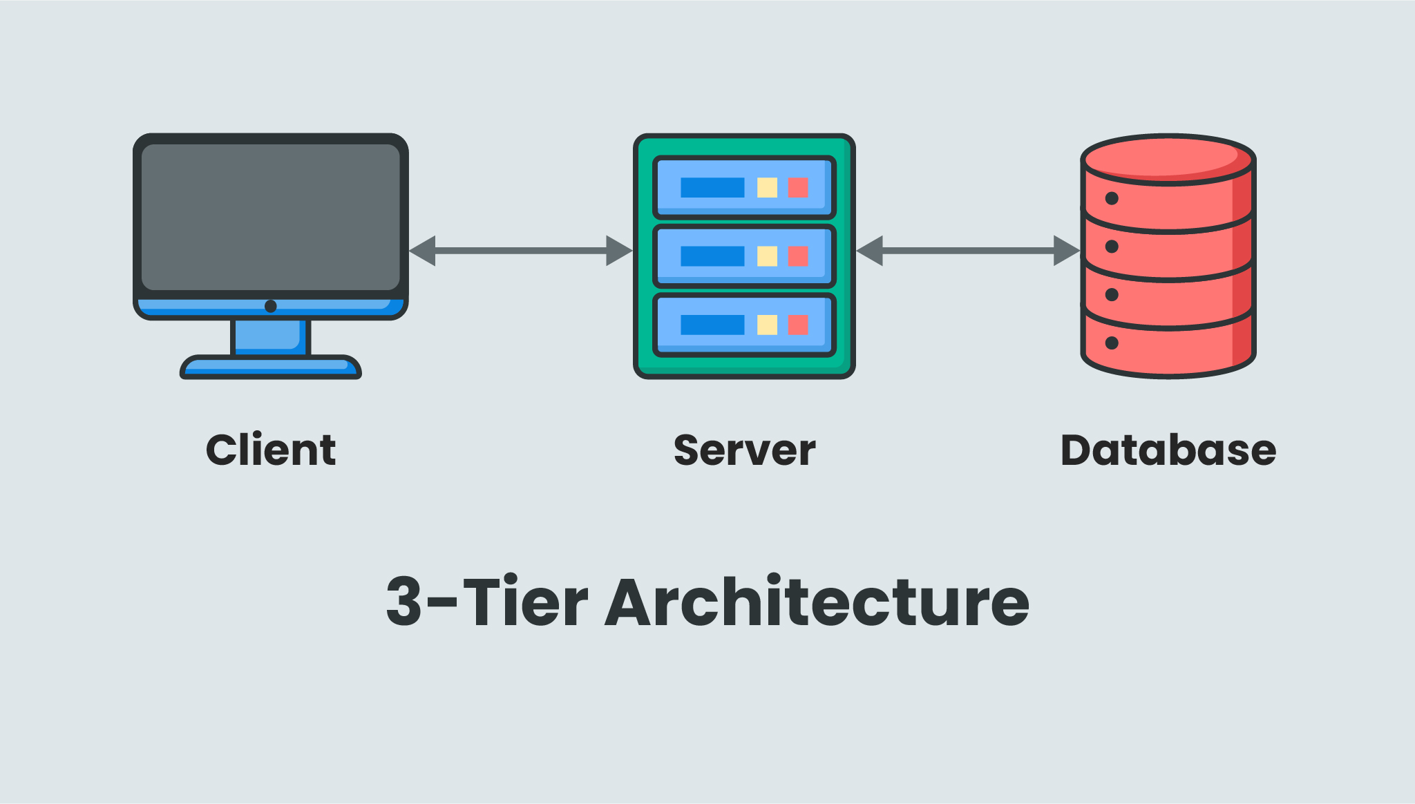
3 Layers: Client (Application) Layer > Application Server / Business Layer > Database Layer
Clients have an interface which allows them to interact with the middleware application server. They don't directly connect to the database server.
Database server does not get overwhelmed since the middleware server handles all the queries, so load on it is reduced.

+ Can be scaled.
+ Secure, since client is not directly interacting with the database server.
- More complex and difficult to maintain compared to 2-Tier architecture.

Schema & 3-Schema Architecture

Image taken from here

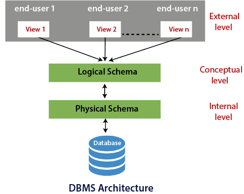
Schema means the logical representation of data in the database. It tells us about the structure in which the data will be stored. We also get information about the elements in the structure, their size, etc.
We're not interested in the physical representation of the data, ie how exactly they're stored in the database. We're only interested in a legible representation of the data.
A 3-Schema architecture consists of 3 levels: View | Logical | Physical
We see data in the form of a table, but it is actually stored in the form of files.

1: External Schema / View Level:

Controlled by the Front-end Developer.
Different types of users (student, faculty, etc.) have different views.
Within a particular type, different users are shown different data, relevant to them, within the particular view.

2: Conceptual Schema / Logical Level:

Controlled by the Database Designer.
Can be called a blueprint of the structure.
Stores information about the tables, and the data in the tables.
Stores Relationships between the tables ie how they are connected.

3: Physical Schema / Physical Level:

Controlled by the Database Administrator.
Stores information about where the data is stored, how it is stored.
Decides if data is centralized or de-centralized.

Data Independence

The actual data is shown to the user, but information about how it is stored, where it is stored, etc. is hidden.
We don't show all the tables to the user, we only show the relevant information the user wants to see.
The application program is not changed, since the user directly interacts with it and it used to the particular view.
The objective is to make changes in the Conceptual and Physical Schema in such a way that the user (View Level) is not affected.
Logical Data Independence:
- Changes made in the Conceptual Schema don't affect the External Schema.
- Example: The WebUI shown to an user is not affected even after making some changes to the Conceptual Schema of a database system.
Physical Data Independence:
- Changes made in the Physical Schema don't affect the Conceptual Schema or the External Schema.
- Example: Changing file structure, physical storage, Indexing, etc don't affect the Conceptual Schema.

Keys

Any piece of data within a tuple in a database, can be called a key.
Keys are of many types: Primary Key, Candidate Key, etc.

Primary & Candidate Key

Any key that can be used to uniquely identify data tuples (or rows) in a database, is called a primary key.
The primary key must be unique. Also, it must not be wrong or have any default value.
It must not be null.
There must only be 1 primary key in a database table (in case of RDB).
Usually, if there's a possibility that the user cannot provide the data for a primary key at this time, it is auto-generated and assigned to the user. For example, registration number, roll number, etc.
The set of all possible keys that can be used as a primary key, is called Candidate Key.
We can have keys who value is null, in the set of Candidate Keys. However, the Unique property must be maintained.

Example:

Roll Number	Registration Number	SName	City	Age	Phone Number
101	REG2022001	Alice	Paris	20	555-1234-5678
102	REG2022002	Bob	London	22	555-1234-5678
103	REG2022003	Charlie	Berlin	21	555-3456-7890
104	REG2022004	David	Tokyo	23	null
105	REG2022005	Emily	Rome	20	555-5678-9012

Here, the candidate keys are: <Roll No, Registration Number, Phone Number>
Among these, Phone number can be null, so it can't be used as a primary key. Any 1 of the other 2 can be used for the purpose.

Foreign Key

An attribute or set of attributes that references to Primary Key of the same table or another table.
It maintains referential integrity.
If 2 tables are related, there will be atleast 1 common column between them. However, it's not necessary for this column to have the same name in both the tables.
Example: Table 1: Student Information

Roll No Name Address

101 Alice Paris

102 Bob London

103 Charlie Berlin

104 David Tokyo

Table 2: Course Information

Course ID Course Name Roll Number

201 Math 101

202 Science 102

203 English 103

204 History 104
- Here, Roll Number of Table 2 is a foreign key, referencing Roll No in Table 1.
- The names of the columns may or may not be unique.
- SQL query for setting a foreign key during table creation:
```
CREATE TABLE StudentInformation (
    RollNo INT PRIMARY KEY,
    Name VARCHAR(20),
    Address VARCHAR(20)
);

CREATE TABLE CourseInformation (
    CourseID INT PRIMARY KEY,
    CourseName VARCHAR(20),
    RollNumber INT,
    FOREIGN KEY (RollNumber) REFERENCES StudentInformation(RollNo)
);
```
- SQL query for setting a foreign key after table creation (CONSTRAINT name can be anything as it's the name of the constraint):
```
ALTER TABLE CourseInformation
    ADD CONSTRAINT FK_StudentInfo_RollNo
    FOREIGN KEY (RollNumber) REFERENCES StudentInformation(RollNo);
```

Referential Integrity

Integrity means consistency of the data across multiple tables. By preserving referential integrity, we aim to ensure consistency among the data across both the referenced (base) & referencing table.

Now, let's check if INSERT, DELETE & UPDATE operations on either of the tables disturbs the Referential Integrity of the data.
Example: Referenced (Base) Table 1: Student Information

Roll No Name Address

101 Alice Paris

102 Bob London

103 Charlie Berlin

104 David Tokyo
- Primary Key: Roll No
Referencing Table 2: Course Information

Course ID Course Name Roll Number

201 Math 101

202 Science 102

203 English 103

204 History 104
- Foreign Key: Roll Number REFERENCES Roll No.
Operations performed on Referenced (Base) Table 1:
- INSERT: No violation
- UPDATE: Possible violation.
  - Updating the Roll No on Table 1 can introduce inconsistency, because the tuple in Table 2 that was referencing to it, now links to nothing.
  - Solution:
    1. Update manually: Recommended.
    2. $onUpdateCascade()$: When Roll No is updated, delete the corresponding row on Table 2. This can result in loss of data.
    3. $onUpdateSetNull()$: When Roll No is updated, set the Roll Number of the corresponding row on Table 2, to null. However, this may cause issues if the foreign key is also a primary key of Table 2.
- DELETE: Possible violation.
  - We may accidentally delete a tuple whose Roll No has been referenced by Table 2.
  - Solution:
    1. No action: Do nothing, this is not recommended for obvious reasons.
    1. $onDeleteSetNull()$: When the tuple is deleted, set the Roll Number of the corresponding row on Table 2, to null.
Operations performed on Referencing Table 2:
- INSERT: Possible violation.
  - We cannot insert a tuple in this table with a Roll Number that doesn't reference to any tuple in Table 1.
  - Solution: Ensure that the corrensponding tuple exists in Table 1.
- UPDATE: Possible violation.
  - Updating the foreign key, Roll Number on Table 2 can introduce inconsistency, while it's fine to update other columns.
  - Solution:
    1. Before updating the foreign key, ensure that it's not referencing to any primary key in Table 1.
- DELETE: No violation.

Super Key

It is a combination of all possible attributes which can uniquely identify 2 tuples in a table. We pair the candidate key with any other key, to uniquely identify the tuple.
A super-set of any candidate key is called a super key.
Example 0: IF $R(A_1,A_2,A_3,...A_n)$:
- If $A_1$ is a candidate key, then how many super keys are possible?
  - Usually, per key, we have 2 choices. We can either include it in our set, or exclude it.
    
    Total number of possible choices in general: $2^n$
  - But, here $A_1$ is said to be the candidate key, and must be included. For the rest, they may or may not be included.
    
    Total number of possible choices: $2^{n-1}$
- If $A_1$ & $A_2$ are candidate keys:
  - If we just take $A_1$, we have $2^{n-1}$ possible choices.
  - If we just take $A_2$, we have $2^{n-1}$ possible choices.
  - However, both these super sets will have some elements in common. For $A_1$ set, we will have elements which contain $A_2$ in them, and vice versa. So, we need to exclude them. We intend to exclude elements which contain both $A_1$ & $A_2$ in them, which is $2^{n-2}$.
    
    Number of possible sets: $2^{n-1}+2^{n-1}-2^{n-2}$
- If $A_1 A_2$ & $A_3 A_4$ are candidate keys:
  
  Similarly, the number of possible sets: $2^{n-2}+2^{n-2}-2^{n-4}$

Data Models

Before implementing a database, we need to draw a logical design for the end-product. This design is called a data model.

Entity Relationship Model

Entity: Object which has some attributes.
Relationship: Relationships among the entities.

Attributes

Example: Student

Single: Attribute which has only 1 value.

Registration number.
Multivalued: has more than 1 values.

Mobile Number

Simple: cannot be broken further

Age
Composite: can be broken further

Name, cab be broken down into first name, middle name, last name
Date of Birth, can be broken down into DD,MM,YY
Address
Complex: Composite + Multivalued

Address, it is composite, and a single student can have multiple addresses too.

Stored: directly stored.

Date of Birth
Derived: derived from stored attribute.

Age, derived from Date of Birth.

Key: can be used as the Primary key in a database.

Registration number
Non-key: All keys other than the key attribute.

Name

Required: mandatorily needs to have a value.

Username, usually.
Optional: may not have a value.

Mobile number, usually.

Relationships

One to One

Representation: 1-1 | One-One
Example:
- 3 tables: Employee, Work, Department
- In Employee: E_id is the primary key
- In Department : D_id is the primary key
- In the Relationship table, Work:
  - Foreign keys:
    - E_id: referencing to E_id of Employee.
    - D_id: referencing to D_id of Department.
  - Relationship (1-1): An employee only works in a single Department.
    - E_id: Value is unique
    - D_id: Value is unique
  - Primary Key: Either of the primary keys of the LHS or RHS table.
    
    Any of E_id or D_id
- We can reduce (merge) Employee & Work into a single Employee table. In fact, we can merge the Relationship table with either the LHS or the RHS table.

One to Many

Representation: 1-M | One-Many
Example:
- 3 tables: Customer, Places, Order
- In Customer: C_id is the primary key
- In Order : O_no is the primary key
- In the Relationship table, Places:
  - Foreign keys:
    - C_id: referencing to C_id of Customer.
    - O_no: referencing to O_no of Order.
  - Relationship (1-Many): A customer can place multiple orders.
    - C_id: Value can repeat
    - O_no: Value is unique
  - Primary Key: Primary key of the RHS table.
    
    O_no, since C_id can repeat.
- We can merge (reduce) Places & Order into a single Order table, ie we're merging the Relationship table with the RHS table.

Many to One

Representation: M-1 | Many-One
Example:
- 3 tables: Order, Placed-by, Customer
- In Order : O_no is the primary key
- In Customer: C_id is the primary key
- In the Relationship table, Placed-by:
  - Foreign keys:
    - O_no: referencing to O_no of Order.
    - C_id: referencing to C_id of Customer.
  - Relationship (Many-1): Many orders can be placed by a single customer.
    - O_no: Value is unique
    - C_id: Value can repeat
  - Primary Key: Primary key of the LHS table.
    
    O_no, since C_id can repeat.
- We can merge (reduce) Placed-by & Order into a single Order table, ie we're merging with the LHS table.

Many to Many

Representation: M-N | Many-Many
Example:
- 3 tables: Student, Study, Course
- In Study : RollNo is the primary key.
- In Course: Cid is the primary key.
- In the Relationship table, Study:
  - Foreign keys:
    - RollNo: referencing to RollNo of Student.
    - C_id: referencing to C_id of Course.
  - Relationship (May-Many): A student can take up multiple courses, and a course can be taken up by multiple students.
    - RollNo: Value can repeat
    - C_id: Value can repeat
  - Primary Key: A composite key, including both the primary keys from the LHS & RHS tables.
    
    RollNo + C_id, since both RollNo & C_id can repeat.
- We cannot merge (reduce) the tables.

Normalization

It is a method of removing or reducing redundancy ie duplicate values from a table.
2 rows cannot be exactly the same, since we have a primary key in every table. At the very least, the primary key column will be different. However, the other values may be partially or fully duplicated.
There are 3 types of anamolies:

Anamoly: Error that only occurs under special circumstances.
- Insertion
- Deletion
- Updation

Example:

$S_{ID}$	Sname	C_ID	Cname	F_ID	Fname	Salary
101	Alice	201	Math	301	John	50000
102	Bob	202	English	302	Emily	55000
103	Charlie	203	Science	303	Sarah	60000
104	Bob	202	English	302	Emily	55000
105	Emma	205	Geography	305	Alex	58000

Insertion Anamoly: We cannot insert a new course in this table, unless there's also a student to take it up, and $S_{ID}$ is a primary key.
Deletion Anamoly: We can delete $S_{ID}=102$ safely without losing data because details for $C_{ID}=202$ & $F_{ID}=302$ is also present in other rows. But, if we delete $S_{ID}=105$, we may lose important information.
Updation Anamoly: Say we want to update the salary of faculty $F_{ID}=302$ ie Emily from $55000$ to $60000$. Now, since there is only 1 faculty with $F_{ID}=302$, the updation should only happen once. But, in reality, since there are multiple entries of $F_{ID}=302$, value $55000$ will be updated multiple times within the table (twice, in this example).

Normalization aims to prevent these anamolies from happening.

Functional Dependency

X -> Y: means that X determines Y, or Y is determined by X.
- X: Determinant
- Y: Dependent Attribute
Example:
- X: Sid, Y: Sname, X -> Y
1. VALID, data has been duplicated.
  
  Sid Sname
  
  1 Ranjit
  
  1 Ranjit
2. VALID, they are different people.
  
  Sid Sname
  
  1 Ranjit
  
  2 Ranjit
3. VALID, they are different people.
  
  Sid Sname
  
  1 Ranjit

So, for the same reason, if a dependency contains in the left part a proper subset of a candidate key plus a non-prime attribute, this does not fall under the Codd’s definition, meaning that it does not violate such definition. |2|Varun| 1. INVALID, Sid cannot be same for different people. |Sid|Sname| |---|---| |1|Ranjit| |1|Varun|

Types:
- Trivial: Functional Dependencies where if (X -> Y), then Y is a subset of X. Also, they are always valid, because effectively, X is determining itself. Example: (Sname,Sid -> Sid).
- Non-Trivial: Functional Dependencies where if (X -> Y), then Y is not a subset of X. Example: (Eid -> Ename).
Properties:
- Reflexivity: If X & Y are Trivial Functional Dependencies (Y is a subset of X), then (X -> Y)
- Augmentation: If (X -> Y), then (XZ -> YZ)
- Transitive: If (X -> Y) & (Y -> Z), then (X -> Z)
- Union: If (X -> Y) & (X -> Z), then (X -> YZ)
- Decomposition: If (X -> YZ), then (X -> Y) & (X -> Z). You cannot Decompose the left hand side.
- Composition: If (X -> Y) & (Z -> W), then (XZ -> YW)
- Pseudotransitivity: If (X -> Y) & (WY -> Z), then (WX -> Z)

Closure Method

A method to find candidate keys from functional dependencies (FDs).
2 methods:
1. One by one: Examples 0,1
2. More efficient: Example 2
Example 0:
- R=(ABCD) | FD = {A->B, B->C,C->D}
- $A^+=ABCD$
- $B^+=BCD$
- $C^+=CD$
- $D^+=D$
- $AB^+=ABCD$, but cannot be considered because candidate keys should be minimal. However, it can be a super key.
- Prime Attributes: ${A}$
These attributes can be used as a candidate key.
- Non-Prime Attributes: ${B,C,D}$
These attributes cannot be used as a candidate key.
- $A$ is included in $A^+$ because it will always determine it's own value.
- Only attributes that determine the values of all attributes in the relation, can be the candidate key.
Example 1:
- R=(ABCD) | FD = {A->B, B->C,C->D,D->A}
- $A^+=ABCD$
- $B^+=BCDA$
- $C^+=CDAB$
- $D^+=DABC$
- Prime Attributes: ${A,B,C,D}$
- Non-Prime Attributes: ${null}$
Example 2:
- R=(ABCDE) | FD = {A->B, BC->D,E->C,D->A}
1. Check the RHS of the functional dependencies: ${AB,D,C,A}$. E is missing, so assume that E will be a part of the candidate key.
2. Start check from `n which the left part is a proper subset of a candidate key and the right part is a non prime attribute.

So, for the same reason, if a dependency contains in the left part a proper subset of a candidate key plus a non-prime attribute, this does not fall under the Codd’s definition, meaning that it does not violate such definition.A: > $AE^+=\{AECBD\}$. Candidate Key Set: $\{AE\}$ 1. Check if AorEis in RHS: \[D->A\]. Check forD: > $DE^+=\{DEABC\}$. Candidate Key Set: $\{AE,DE\}$ 1. Check if Dis in RHS: \[BC->D\]. Check forB&C`: > $BE^+={BECDA}$. Candidate Key Set: ${AE,DE,BE}$
> $CE^+={CE}$. Candidate Key Set: ${AE,DE,BE}$ - So, in short, when we find a new candidate key, we search if that new attribute is also present in RHS of the FD. If it is, we check for the corresponding LHS attributes.

First Normal form (1-NF)

The table should not contain multivalued attributes.
Example: Normalize this table to 1-NF (Solution 3 is the one that works):

RollNo Name Course

1 Sai C,C++

2 Harsh Java

3 Onkar C,DBMS
- Solution 1: Put only 1 course per row.
  
  RollNo Name Course
  
  1 Sai C
  
  1 Sai C++
  
  2 Harsh Java
  
  3 Onkar C
  
  3 Onkar DBMS
  - Primary Key: RollNo+Course
```
- Data Duplication
```
- Solution 2: Divide the Course column:
  
  RollNo Name Course 1 Course 2
  
  1 Sai C C++
  
  2 Harsh Java null
  
  3 Onkar C DBMS
  - Primary Key: RollNo
  - null: no value
```
- If there are 2 columns for course & someone takes up a 3rd course, we have to add another column for `Course 3`.
- For people who have only taken 1 course, we have to put the value for course 2,3,... n as `null`, which is not good practice.
```
- Solution 3: Segregate into 2 tables.
  - Base Table
    
    RollNo Name
    
    1 Sai
    
    2 Harsh
    
    3 Onkar
    - Primary Key: RollNo
  - Referencing Table:
    
    RollNo Course
    
    1 C
    
    1 C++
    
    2 Java
    
    3 C
    
    3 DBMS
  - Primary Key: RollNo+Course
  - Foreign Key: RollNo, referencing to RollNo.

Second Normal form (2-NF)

Table must be in First Normal Form (1-NF).
All the non-prime attributes must be fully functionally dependent on the Candidate Key. They must not be only partially dependent on a part of (ie a proper subset of) the Candidate Key.
It's not a problem if both LHS and RHS are non-prime attributes.
(AB -> C) should happen.
If (AB -> C), AB is a candidate key (prime attribute) while C is a non-prime attribute. If (A -> C) or (B -> C) is true, then the table is not in 2-NF.
Example:

Customer ID Store ID Location

1 1 Delhi

1 3 Mumbai

2 1 Delhi

3 2 Bangalore

4 3 Mumbai
- Primary Key: Customer ID + Store ID
- Here, Location (non-prime attribute), is only dependent on one of the prime attributes (Store ID). So, it's not in 2-NF.
- So, we divide it into 2 tables.
- Table 1 (no dependency problems):
  
  Customer ID Store ID
  
  1 1
  
  1 3
  
  2 1
  
  3 2
  
  4 3
- Table 2 (Location is dependent on the only prime attribute, Store ID):
  
  Store ID Location
  
  1 Delhi
  
  2 Bangalore
  
  3 Mumbai
Example 1:
- $R={A,B,C,D,E,F}$, FD: {C->F, E->A, EC->D, A->B}
1. Here, C & E are not present in the RHS of the functional dependencies. So, let's check for $CE^+$.
2. $CE^+={CEAFDB}$
3. Candidate Key: CE
4. None of C,E are present in the RHS of the functional dependencies, so {CE} is the only candidate key.
5. Prime attributes: ${C,E}$
6. Non-Prime attributes: ${A,B,D,F}$
7. Here,because C->F, E->A, we can clearly see the C & E by tehmselves are determining a non-prime attribute. So, table is not in 2-NF.

Third Normal form (3-NF)

Table must be in Second Normal Form (2-NF).
Table must not have any Transitive Dependency. For (X->Y), X should be a Candidate Key, or Y should be a prime attribute.
If AB -> CD, and D -> A:
- Candidate Keys: {AB,DB}
- Prime Attributes: {A,B,D}
- Non-prime Attributes: {C)
- Among the Functional Dependencies, none have any Transitive Dependency.

Boyce Codd Normal Form (BCNF)

A special case of 3rd Normal Form.
Table must be in Third Normal Form (3-NF).
The left hand side of each functional dependency should be a candidate key or super key.
3-NF preserves dependencies, but BCNF does not.
However, BCNF ensures Lossless Decomposition.
Example 0:
- Candidate Keys: {RollNo, VoterID}
- Functional Dependencies:
  - RollNo -> Name
  - RollNo -> VoterID
  - VoterID -> Age
  - VoterID -> RollNo
- All are valid, since the LHS attributes are all prime attributes.
Example 1: R(ABCD)
- AB -> CD
- D -> A
1. Candidate Keys: {AB,DB}
2. Prime Attributes: {A,B,D}
3. Non-Prime Attributes: {C}
4. Here, in {D -> A}, D is not a candidate key. So the table is not in BCNF. Let's convert it into BCNF.
5. We separate DA since {D -> A} was the problem.
6. We also separate BCD.
7. So, ABCD -> DA,BCD
8. Lossless Decomposition: The attribute that is common to both tables will be the candidate key of the tables individually, or both of them.
9. Now, generate the Functional Dependencies: D -> A, BD -> C.
10. Here, {AB -> CD} is not preserved. So, the fact that BCNF does not preserve dependencies, is proved.

4th Normal Form (4-NF)

Table must be in Boyce Codd Normal Form.
No multivalued dependencies must be present.

Example:

If a person has 3 mobile numbers and 3 E-Mail ID's, this is what the table will look like:

Name	Mobile Number	E-Mail
John	1111111111	aa@aa.com
John	1111111111	bb@bb.com
John	1111111111	cc@cc.com
John	2222222222	aa@aa.com
John	2222222222	bb@bb.com
John	2222222222	cc@cc.com
John	3333333333	aa@aa.com
John	3333333333	bb@bb.com
John	3333333333	cc@cc.com

Our main with Normalization is to reduce redundancy in the data, so we must not have any multivalued dependency like this.

5th Normal Form (5-NF)

The Decomposition must be Lossless in nature.
If, after joining the tables to get back the original table, we see that the Decomposition was Lossless, we can be sure that the table is in 5-NF.
There will be no difference between the tuples in our table and the original table.

Decomposition

Lossy Decomposition: Decomposition that leads to inconsistency in data.
When Decomposing a table, the common attribute should be the candidate key of either of the tables, or both of them. This ensures Lossless Decomposition.
Example 0 (Lossy Decomposition):
- Table $R$:
  
  A B C
  
  1 2 1
  
  2 2 2
  
  3 3 2
- Table $R_1$:
  
  A B
  
  1 2
  
  2 2
  
  3 3
- Table $R_2$:
  
  B C
  
  2 1
  
  2 2
  
  3 2
- Question: Find the value of C if A: 1.
- Query: Select $R_2C\ from\ R_2\ NATURAL\ JOIN\ R_1, WHERE\ R_1 A=1$
1. First, find the cross product of all rows of the tables.
  
  A B B C
  
  1 2 2 1
  
  1 2 2 2
  
  1 2 3 2
  
  2 2 2 1
  
  2 2 2 2
  
  2 2 3 2
  
  3 3 2 1
  
  3 3 2 2
  
  3 3 3 2
2. Remove the rows where the value of B is different.
  
  A B B C
  
  1 2 2 1
  
  1 2 2 2
  
  2 2 2 1
  
  2 2 2 2
  
  3 3 3 2
3. The Natural Join table is:
  
  A B C
  
  1 2 1
  
  1 2 2
  
  2 2 1
  
  2 2 2
  
  3 3 2
4. We can clearly see that C is resolving to 1 & 2 for A=1.
5. We can also see that the number of rows is more in this table, compared to the original table R.
6. The extra tuples are called Spurious Tuples.
Example 1 (Lossless Decomposition):
- Table $R$:
  
  A B C
  
  1 2 1
  
  2 2 2
  
  3 3 2
- Table $R_1$:
  
  A B
  
  1 2
  
  2 2
  
  3 3
- Table $R_2$:
  
  A C
  
  1 1
  
  2 2
  
  3 2
- As we see, there are no Spurious Tuples when using A as the common attribute, following the above rule.
- Example 1: Check if Functional Dependencies are preserved:
  - R(ABCD)
  - Functional Dependencies: { A->B, B->C, C->D, D->B }
  - R is decomposed into $R_1(AB)$, $R_2(BC)$, $R_1(BD)$.
  1. Check if any attributes have been left out in the decomposed tables: false, they're intact.
  2. Check for all possible non-trivial dependencies of the decomposed tables, with respect to the original Functional Dependencies:
    
    $R_1(AB)$ $R_2(BC)$ $R_3(BD)$
    
    {A->B} {B->C} {B->D}
    
    ~~{B->A}~~ {C->B} {D->B}
  3. So, dependencies are: { A->B, B->C, B->D, C->B, D->B }.
  4. Now, check if these dependencies include all the ones in the original Functional Dependency.
    - { A->B }: true
    - { B->C }: true
    - { C->D }: true
    - { D->B }: true
  5. So, functional dependencies are preserved.
- Example 2: Check if Functional Dependencies are preserved:
  - R(ABCD)
  - Functional Dependencies: { AB->CD, D->A }
  - R is decomposed into $R_1(AD)$, $R_2(BCD)$
  1. Check if any attributes have been left out in the decomposed tables: false, they're intact.
  2. Check for all possible non-trivial dependencies of the decomposed tables, with respect to the original Functional Dependencies:
    
    $R_1(AD)$ $R_2(BCD)$
    
    ~~{A->D}~~ ~~{B->C}~~
    
    {D->A} ~~{C->D}~~
    
    null ~~{D->B}~~
    
    null ~~{BC->D}~~
    
    null ~~{CD->B}~~
    
    null {BD->C}
  3. So, dependencies are: { D->A, BD->C }
  4. Now, check if these dependencies include all the ones in the original Functional Dependency.
    - { AB->CD }: false
    - { D->A }: true
  5. So, functional dependencies are not preserved.

Minimal Cover

The aim is to reduce or simplify the Functional Dependencies.
Example: For the following Functional Dependencies, find the correct Minimal Cover: {A->B,C->B,D->ABC,AC->D}
1. Simplify the dependencies: {A->B,C->B,D->A,D->B,D->C,AC->D}
2. Remove the functional dependencies one by one, and check if that results in loss of dependencies (false: cannot be removed).
  1. (A->B), $A^+=A$, false
  2. (C->B), $C^+=C$, false
  3. (D->A), $D^+=DBC$, false
  4. (D->B), $D^+=DABC$, true
  5. (D->C), $D^+=DAB$, false
  6. (AC->D), $AC^+=ACB$, false
3. Only (D->B) can be removed.
4. So, current dependencies: {A->B,C->B,D->A,D->C,AC->D}
5. Now, check if the left side of the dependencies can be minimized further. Try to keep only 1 attribute on the LHS, and see if you can get the other attributes in it's closure.
  1. (AC->D), $A^+=AB$, $C^+=CB$, false
  2. After removing A, we're trying to get $A$ in $C^+$, and after removing C, we're trying to get $C$ in $A^+$.
6. Minimal list of Dependencies: {A->B,C->B,D->A,D->C,AC->D}

Normalization Examples

Example 0: $R(ABCDEF)$, Functional Dependencies: ${AB->C,C->DE,E->F,F->A}$, Check the highest Normal Form.
1. Find the Candidate Keys.
  1. ${AB^+=ABCDEF}$, true
  2. A is present in RHS for (F->A). So, ${FB^+=FBACDE}$, true
  3. F is present in RHS for (E->F). So, ${EB^+=EBFACD}$, true
  4. E is present in RHS for (C->DE). So, ${CB^+=CBDEFA}$, true
  5. C is present in RHS for (AB->C), but AB has already been defined.
  6. Candidate Keys: ${AB,FB,EB,CB}$
2. Note the Prime Attributes: ${A,B,C,E,F}$
3. Note the Non-Prime Attributes: ${D}$
4. Check for Normal Form (1: valid):
  
  Normal Form AB->C C->DE E->F F->A
  
  BCNF 1 0 0 0
  
  3-NF 1 0 1 1
  
  2-NF 1 0 1 1
  
  1-NF 1 1 1 1
  - Check in reverse order, starting with BCNF.
  - For 1-NF, whether the attributes are multivalued or not cannot be determined, so we assume that the table is atleast in 1-NF.
Example 1: $R(ABCDEF)$, Functional Dependencies: ${AB->C,C->D,C->E,E->F,F->A}$, Convert the table to BCNF.
- Candidate Keys: ${AB,FB,EB,CB}$
- Prime Attributes: ${A,B,C,E,F}$
- Non-Prime Attributes: ${D}$
- Functional Dependencies: ${AB->C,C->D,C->E,E->F,F->A}$
1. Check for 1-NF: We cannot check for atomicity here, since we need the attribute values to do so. We assume that the table is already in 1-NF.
2. Check for 2-NF:
  - (AB->C): true
  - (C->D): false
  - (C->E): true
  - (E->F): true
  - (F->A): true
  - In (C->D), a non-prime attribute is being determined by a part of the candidate key.
  1. Divide the table into two. Separate the dependency that is causing a problem.
  2. $R_1=ABEF$, $R_2=CD$
  3. Here, we need to have atleast 1 variable common.
  4. In $R_2$, $C^+=CD$ ie C is a candidate key. So, we can use C as a common variable.
  5. $R_1=ABCEF={AB->C,C->E,E->F,F->A}$, $R_2=CD={C->D}$
3. Check for 3-NF:
  1. $R_1$, Candidate Keys: {AB,FB,EB,CB}:
    - (AB->C): true
    - (C->E): true
    - (E->F): true
    - (F->A): true
  2. $R_2$, Candidate Keys: {C}:
    - (C->D): true
4. Check for BCNF:
  1. $R_1$, Candidate Keys: {AB,FB,EB,CB}:
    - (AB->C): true
    - (C->E): false
    - (E->F): false
    - (F->A): false
  2. $R_2$, Candidate Keys: {C}:
    - (C->D): true
  3. We have to Decompose $R_1$.
    - $R_3=(AB->C)=ABC$, Candidate Key: {AB} (from existing)
    - $R_4=(C->E)=CE$, Candidate Key: {C}
    - $R_5=(E->F)=EF$, Candidate Key: {E}
    - $R_6=(F->A)=FA$, Candidate Key: {F}
Example 2: Which of the following statement is true?
- A relation is in 3-NF, then it is always in BCNF.
- A relation is in 2-NF, then it is not in 1-NF.
- A relation is in BCNF, then it is in 2-NF.
- A relation is in 2-NF, it contains partial dependencies.
Example 3: Relation R has 8 attributes, $R=ABCDEFGH$. Functional Dependencies: ${CH->G,A->BC,B->CFH,E->A,F->EG}$
1. D is not present in RHS.
2. $DA^+=DABCFHGE$ | Candidate Keys: ${DA}$
3. A is on the RHS of (E->A). Check for E.
4. $DE^+=DEABCFHG$ | Candidate Keys: ${DA,DE}$
5. E is on the RHS of (F->EG). Check for F.
6. $DF^+=DFEGABCH$ | Candidate Keys: ${DA,DE,DF}$
7. F is on the RHS of (B->CFH). Check for B.
8. $DB^+=DBCFHEGA$ | Candidate Keys: ${DA,DE,DF,DB}$
9. So, total number of candidate keys: $4$.
Example 3: Check the highest Normal Forms for these tables:
- Schema 1:
  - Registration (rollno, courses)
  - Functional Dependencies: {rollno -> courses}
  1. BCNF:
    - { rollno -> courses }: true
- Schema 2:
  - Registration (rollno, courseid, email)
  - Functional Dependencies: {rollno, courseid -> email, email -> rollno}
  1. BCNF:
    - { rollno,courseid -> email }: true
    - { email -> rollno }: false
  2. 3-NF:
    - { rollno,courseid -> email }: true
    - { email -> rollno }: true
- Schema 3:
  - Registration (rollno, courseid, marks, grade)
  - Functional Dependencies: {rollno,courseid -> marks, grade, marks -> grade}
  1. BCNF:
    - { rollno, courseid -> marks, grade }: true
    - { marks -> grade }: false
  2. 3-NF:
    - { rollno, courseid -> marks, grade }: true
    - { marks -> grade }: false
  3. 2-NF:
    - { rollno, courseid -> marks, grade }: true
    - { marks -> grade }: true
- Schema 4:
  - Registration (rollno, courseid, credit)
  - Functional Dependencies: {rollno, courseid -> credit, courseid -> credit}
  1. BCNF:
    - { rollno, courseid -> credit }: true
    - { courseid -> credit }: false
  2. 3-NF:
    - { rollno, courseid -> credit }: true
    - { courseid -> credit }: false
  3. 2-NF:
    - { rollno, courseid -> credit }: true
    - { courseid -> credit }: false
  4. 1-NF:
    - { rollno, courseid -> credit }: true (assumed)
    - { courseid -> credit }: true (assumed)
Equivalence of Functional Dependency
- If the closure of all attributes are same between 2 Functional Dependencies, we can say that they are equivalent to each other.
- Example 0:
  - X = { A->B, B->C}
  - Y = { A->B, B->C, A->C}
  1. Take the LHS attributes of Y one by one, form the closure from X, match with Y:
    - $A^+=ABC$: true
    - $B^+=BC: true
  2. Take the LHS attributes of X one by one, form the closure from Y, match with X:
    - $A^+=ABC$: true
    - $B^+=BC: true
  3. Since both match, X is equivalent of Y.
- Example 1:
  - X = { AB->CD, B->C, C->D }
  - Y = { AB->C, AB->D,C->D }
  1. Take the LHS attributes of Y one by one, form the closure from X, match with Y:
    - $AB^+=ABCD$: true
    - $C^+=CD$: true
  2. Take the LHS attributes of X one by one, form the closure from Y, match with X:
    - $AB^+=ABCD$: true
    - $B^+=BCD$: false
    - $C^+=CD$: true
  3. X is not equivalent of Y.

Joins

Natural Join / Inner Join

Joined table only contains rows where the primary key & foreign key are equal.
Table emp:

Eno Ename Address

1 Alice 123 Main St

2 Bob 456 Elm St

3 Charlie 789 Oak St

4 David 321 Maple St

5 Eve 654 Pine St
Table dept:

DEPTno Name Eno

101 Sales 1

102 HR 2

103 IT 3

104 Finance 4

105 Marketing 5

Cross Product (every row of emp is multiplied with the whole of dept):

Eno	Ename	Address	DEPTno	Name	Eno
1	Alice	123 Main St	101	Sales	1
1	Alice	123 Main St	102	HR	2
1	Alice	123 Main St	103	IT	3
1	Alice	123 Main St	104	Finance	4
1	Alice	123 Main St	105	Marketing	5
2	Bob	456 Elm St	101	Sales	1
2	Bob	456 Elm St	102	HR	2
2	Bob	456 Elm St	103	IT	3
2	Bob	456 Elm St	104	Finance	4
2	Bob	456 Elm St	105	Marketing	5
3	Charlie	789 Oak St	101	Sales	1
3	Charlie	789 Oak St	102	HR	2
3	Charlie	789 Oak St	103	IT	3
3	Charlie	789 Oak St	104	Finance	4
3	Charlie	789 Oak St	105	Marketing	5
4	David	321 Maple St	101	Sales	1
4	David	321 Maple St	102	HR	2
4	David	321 Maple St	103	IT	3
4	David	321 Maple St	104	Finance	4
4	David	321 Maple St	105	Marketing	5
5	Eve	654 Pine St	101	Sales	1
5	Eve	654 Pine St	102	HR	2
5	Eve	654 Pine St	103	IT	3
5	Eve	654 Pine St	104	Finance	4
5	Eve	654 Pine St	105	Marketing	5

Example 0: Select Ename from emp natural join dept

Explanation: Select Ename from emp,dept where emp.Eno=dept.Eno

Values:

Eno	Ename	Address	DEPTno	Name	Eno
1	Alice	123 Main St	101	Sales	1
2	Bob	456 Elm St	102	HR	2
3	Charlie	789 Oak St	103	IT	3
4	David	321 Maple St	104	Finance	4
5	Eve	654 Pine St	105	Marketing	5

Answer: Alice, Bob, Charlie, David, Eve

Self Join

Here, we join a table with itself.

Example 0: Select Sid from study as t1, study as t2 where t1.Sid=t2.Sid and t1.Cid < > t2.Cid

Explanation: Select Sid, where student has taken up atleast 2 courses. { < > means not equal }
Table study:

Sid Cid Since

$S_1$ $C_1$ 2016

$S_2$ $C_2$ 2017

$S_1$ $C_2$ 2017

Cross-Product (with itself):

Sid	Cid	Sid	Cid	Since
$S_1$	$C_1$	$S_1$	$C_1$	2016
$S_1$	$C_1$	$S_2$	$C_2$	2017
$S_1$	$C_1$	$S_1$	$C_2$	2017
$S_2$	$C_2$	$S_1$	$C_1$	2016
$S_2$	$C_2$	$S_2$	$C_2$	2017
$S_2$	$C_2$	$S_1$	$C_2$	2017
$S_1$	$C_2$	$S_1$	$C_1$	2016
$S_1$	$C_2$	$S_2$	$C_2$	2017
$S_1$	$C_2$	$S_1$	$C_2$	2017

Values:

Sid Cid Sid Cid Since

$S_1$ $C_1$ $S_1$ $C_2$ 2017

$S_1$ $C_2$ $S_1$ $C_1$ 2016
Answer: Sid

Equi & Non-Equi Join

Table emp:

Eno Ename Address

1 Alice 123 Main St

2 Bob 456 Elm St

3 Charlie 789 Oak St

4 David 321 Maple St

5 Eve 654 Pine St
Table dept:

DEPTno Location Eno

101 123 Main St 1

102 456 Elm St 2

103 789 Oak St 3

104 777 Maple St 4

105 654 Pine St 5

Cross Product (every row of emp is multiplied with the whole of dept):

Eno	Ename	Address	DEPTno	Location	Eno
1	Alice	123 Main St	101	123 Main St	1
1	Alice	123 Main St	102	456 Elm St	2
1	Alice	123 Main St	103	789 Oak St	3
1	Alice	123 Main St	104	777 Maple St	4
1	Alice	123 Main St	105	654 Pine St	5
2	Bob	456 Elm St	101	123 Main St	1
2	Bob	456 Elm St	102	456 Elm St	2
2	Bob	456 Elm St	103	789 Oak St	3
2	Bob	456 Elm St	104	777 Maple St	4
2	Bob	456 Elm St	105	654 Pine St	5
3	Charlie	789 Oak St	101	123 Main St	1
3	Charlie	789 Oak St	102	456 Elm St	2
3	Charlie	789 Oak St	103	789 Oak St	3
3	Charlie	789 Oak St	104	777 Maple St	4
3	Charlie	789 Oak St	105	654 Pine St	5
4	David	321 Maple St	101	123 Main St	1
4	David	321 Maple St	102	456 Elm St	2
4	David	321 Maple St	103	789 Oak St	3
4	David	321 Maple St	104	777 Maple St	4
4	David	321 Maple St	105	654 Pine St	5
5	Eve	654 Pine St	101	123 Main St	1
5	Eve	654 Pine St	102	456 Elm St	2
5	Eve	654 Pine St	103	789 Oak St	3
5	Eve	654 Pine St	104	777 Maple St	4
5	Eve	654 Pine St	105	654 Pine St	5

Equi Join: Condition checks are for equality.
- Query: Select Ename from emp,dept where emp.Eno=dept.Eno and emp.Address=dept.Location
- Explanation: Select Ename where the address & locations match in both tables.
- Filtered table:
  
  Eno Ename Address DEPTno Location Eno
  
  1 Alice 123 Main St 101 123 Main St 1
  
  2 Bob 456 Elm St 102 456 Elm St 2
  
  3 Charlie 789 Oak St 103 789 Oak St 3
  
  5 Eve 654 Pine St 105 654 Pine St 5
- Answer: Alice, Bob, Charlie, Eve
Non-Equi Join: Condition checks are for in-equality.
- Query: Select Ename from emp,dept where emp.Eno=dept.Eno and dept.DEPTno>102
- Explanation: Select Ename where the DEPTno is greater than 102.
- Filtered table:
  
  Eno Ename Address DEPTno Location Eno
  
  3 Charlie 789 Oak St 103 789 Oak St 3
  
  4 David 321 Maple St 104 777 Maple St 4
  
  5 Eve 654 Pine St 105 654 Pine St 5

Left-Outer, Right-Outer & Full-Outer join

Table emp:

EMPno Ename DEPTno

101 Alice 101

102 Bob 102

103 Charlie 101

104 David 104
Table dept:

DEPTno Dname Loc

101 Sales New York

102 HR Los Angeles

103 IT Chicago

104 Finance San Francisco

105 Marketing Boston
Left-Outer Joined Table:
- Keeping the primary & foreign key equal, it gives all the rows in the left table, and corresponding rows in the right table.
- Query: Select EMPno, Ename, DEPTno, Dname, Loc from emp left outer join dept on (emp.DEPTno=dept.DEPTno)
- Table:
  
  EMPno Ename DEPTno Dname Loc
  
  101 Alice 101 Sales New York
  
  102 Bob 102 HR Los Angeles
  
  103 Charlie 101 Sales New York
  
  104 David 104 Finance San Francisco

Right-Outer Joined Table:

Query: Select EMPno, Ename, DEPTno, Dname, Loc from emp right outer join dept on (emp.DEPTno=dept.DEPTno)
Keeping the primary & foreign key equal, it gives all the rows in the right table, and corresponding rows in the left table.

Table:

DEPTno	Dname	Loc	EMPno	Ename
101	Sales	New York	101	Alice
101	Sales	New York	103	Charlie
102	HR	Los Angeles	102	Bob
103	IT	Chicago	null	null
104	Finance	San Francisco	104	David
105	Marketing	Boston	null	null

Full-Outer Joined Table:

Query: Select EMPno, Ename, DEPTno, Dname, Loc from emp full outer join dept on (emp.DEPTno=dept.DEPTno)

Table:

EMPno	Ename	DEPTno	Dname	Loc
101	Alice	101	Sales	New York
102	Bob	102	HR	Los Angeles
103	Charlie	101	Sales	New York
104	David	104	Finance	San Francisco
null	null	103	IT	Chicago
null	null	105	Marketing	Boston

Name	Mobile Number	E-Mail
John	1111111111	[email protected]
John	1111111111	[email protected]
John	1111111111	[email protected]
John	2222222222	[email protected]
John	2222222222	[email protected]
John	2222222222	[email protected]
John	3333333333	[email protected]
John	3333333333	[email protected]
John	3333333333	[email protected]

$R_1(AD)$	$R_2(BCD)$
~~{A->D}~~	~~{B->C}~~
{D->A}	~~{C->D}~~
null	~~{D->B}~~
null	~~{BC->D}~~
null	~~{CD->B}~~
null	{BD->C}

Sid	Sname
1	Ranjit
1	Ranjit

Sid	Sname
1	Ranjit
2	Ranjit

RollNo	Name	Course
1	Sai	C,C++
2	Harsh	Java
3	Onkar	C,DBMS

RollNo	Name	Course
1	Sai	C
1	Sai	C++
2	Harsh	Java
3	Onkar	C
3	Onkar	DBMS

Files

Database-Systems.md

Latest commit

History

Database-Systems.md

File metadata and controls

Questions

qs-UGC_NET-2018

qs-GATE-2005

Basics

Structured data

Unstructured data:

File System vs DBMS

2-Tier Architecture

3-Tier Architecture:

Schema & 3-Schema Architecture

1: External Schema / View Level:

2: Conceptual Schema / Logical Level:

3: Physical Schema / Physical Level:

Data Independence

Keys

Primary & Candidate Key

Foreign Key

Referential Integrity

Integrity means consistency of the data across multiple tables. By preserving referential integrity, we aim to ensure consistency among the data across both the referenced (base) & referencing table.

Super Key

Data Models

Entity Relationship Model

Attributes

Relationships

One to One

One to Many

Many to One

Many to Many

Normalization

Functional Dependency

Closure Method

First Normal form (1-NF)

Second Normal form (2-NF)

Third Normal form (3-NF)

Boyce Codd Normal Form (BCNF)

4th Normal Form (4-NF)

5th Normal Form (5-NF)

Decomposition

Minimal Cover

Normalization Examples

Equivalence of Functional Dependency

Joins

Natural Join / Inner Join

Self Join

Equi & Non-Equi Join

Left-Outer, Right-Outer & Full-Outer join