Home

Reservoir Computing for .NET (RCNet)

The aim of the RCNet is to make the reservoir computing methods easy to use and freely available for .net platform without dependency on other libraries. Two main reservoir computing methods are called Echo State Network (ESN) and Liquid State Machine (LSM). RCNet supports both of these methods. However, since ESN and LSM are based on very similar principles, RCNet brings the option to combine them at the same time. This approach, as I believe, opens up new interesting possibilities. This general implementation is called "State Machine" in the context of RCNet.

This project honors the following:

• Independence. RCNet has and will have all the functionality implemented internally
• Simplicity. Inheritance, polymorphism and interfaces are used only where it is really needed. The simplicity of the code is preferred
• Source code standards. The standard naming convention is used (the only exception is that the fields have an underscore prefix). Source code is fully commented for easy understanding
• Component design. Wherever it is reasonable, the solution is decomposed into generic, reusable components
• Xml parameterization. Each component that is a part of the StateMachine parameterization implements its own corresponding settings class providing initialization parameters. Component must implement public constructor requiring instance of the settings class as a parameter. Settings class has to have defined corresponding initialization xml element type in RCNetTypes.xsd used to validate instance of xml element passed to the constructor
• Serializability. All state components that are required for StateMachine operation are serializable
• Parallel processing. Where appropriate, parallel processing is implemented to achieve better performance

Reservoir Computing conceptual view

Recurrent neural networks (RNNs) are very well suited for processing time-dependent data such as

• Forecasting the next evolution of a time series
• Classification based on time series data Time series can be multivariate.

Examples:

• Based on historical share's prices, forecast its next price
• Based on EEG data, recognize coming epileptic seizure
• Based on voice data, recognize speaker's emotion
• Based on real time micro-movements of the car in the parallel lane, what is the probability that the driver of that car will turn into my lane at the next 3 seconds?
• etc.

Reservoir computing makes it possible to use the benefits of the recurrent network very efficiently. Efficiency lies in the fact that the weights of synapses within the recurrent network (called reservoir) are randomly chosen at the beginning and in contrast with traditional training methods for RNNs, there is no need of any further expensive learning session to find appropriate weights solving given problem. Only the Readout layer is trained, most often very simply, by the quick linear regression.

Figure explanation

• The input data is continuously pushed into the reservoir through input neurons (yellow balls). Input neuron is very simple, it only mediates external input for input synapses (yellow arrows) delivering input to the reservoir's hidden neurons (blue balls interconnected by blue arrows). Each pushed input data starts recomputation cycle of the reservoir.
  • During the recomputation cycle is computed new state of all hidden neurons. Each hidden neuron gets and processes input stimulation using its activation function. Input stimulation of the hidden neuron consists of summed weighted outputs (signals) from connected input neurons and hidden neurons. Recurrently connected hidden neurons do the nonlinear transformation and provide reservoir's dynamics.
  • After each recomputation cycle, the historical and current input data are described by the current state of the reservoir neurons.
• States of reservoir's neurons are so-called predictors. Predictors are periodically collected (mostly after each recomputation cycle) and sent to the readout layer to compute desired output.

Input neuron

Input neuron has associated no activation function and is very simple. Its purpose is only to mediate external input and facilitate its delivery into the reservoir's hidden neurons through synapses.

Synapse

Synapse interconnects two neurons, ensuring unidirectional transmission of weighted signal from source neuron to target neuron. If the signal is always weighted by a constant weight, we are talking about a static synapse. If the weight changes over the time depending on dynamics of connected neurons, we are talking about a dynamic synapse. Synapse can also delay the signal, usually proportionally to the length of the synapse.

Hidden neuron and its Activation function

In general, neuron is a small computing unit that processes the input signal (stimulation) and produces an output signal. The way neuron processes the input signal to output signal defines its so-called Activation function. Neuron can be simply understood as the envelope of its Activation function, where the neuron provides necessary interface and the Activation function performs the core calculations. Activation functions (and therefore also neurons) are distinguished into two types: Analog and Spiking. For a better insight into the activation functions, look at the wiki pages.

Analog activation function

Analog activation function has no similarity to behavior of the biological neuron. It is always stateless, which means that the output value (signal) does not depend on the previous inputs but only on current input at the time T and particular transformation equation (usually non-linear).
A typical example of the analog activation function is TanH (hyperbolic tangent), which non-linearly transforms the input value to the output in the range (-1, 1).

Spiking activation function

Spiking activation function attempts to simulate the behavior of a biological neuron that accumulates (integrates) input stimulation on its membrane potential and when the critical threshold is exceeded, fires a short pulse (spike), resets membrane and the cycle starts from the beginning. In other words, the function implements one of the so-called Integrate and Fire neuron models. For a better insight into the biological neuron models, look at the wiki pages.
It is obvious that spiking activation function is time-dependent and must remember its previous state. The following figure illustrates the progress of membrane potential under constant stimulation. The figure is from the great online book Neuronal Dynamics and shows the behavior of the "Adaptive Exponential Integrate and Fire" model (class AdExpIF in RCNet).

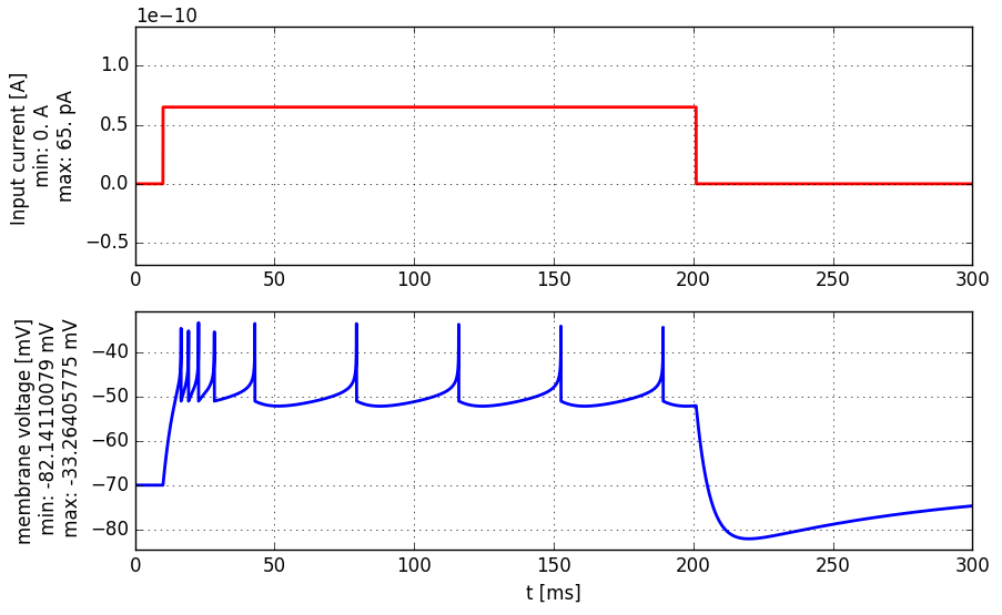
Note that the membrane potential (blue line) is not an output signal. The output signal consists of nine short constant pulses (spikes) at time points where membrane potential exceeds the firing threshold -40 mV. So the output is a zero signal and only at firing times the signal has a value of 1.

Readout layer

Readout layer provides computation of one or more outputs (results) according to given predictors. Before the usage, each output has to be trained using one of the so-called supervised training method. The most commonly used technique is linear regression where linear coefficients are searched that best directly map the predictors to the corresponding desired output values.

Summary notes

• Reservoir is simply the data preprocessor and typically contains hundreds (and sometimes thousands) of recurrently synaptically connected hidden neurons.
• The influence of historical input data on the current states of hidden neurons is weakening in time. The memory capacity of the reservoir depends on several aspects, such as the number of hidden neurons, the type and settings of hidden neurons, the density of the interconnection, synaptic signal delays, ...
• The rich reservoir dynamics allows to train readout layer to map the same predictors to the different outputs (predictions) at the same time. The most commonly used training method is linear regression

Simplified training scenario:

1. Collect all known input and desired corresponding output data
2. Through reservoir, transform the collection of input data into a collection of predictors
3. Train readout layer to be able to compute desired output data from the predictors

Simplified use scenario of the trained network:

1. Get next known input data
2. Through reservoir, transform the input data into the predictors
3. Push predictors into the readout layer and let it to compute output data

--> Next page