P8_rasterPackageAdvanced_II-v1.Rmd

---
title: "P8 Advanced techniques with raster data (part-2) - Supervised Classification"
author: "João Gonçalves"
date: "28 de Novembro de 2017"
output: 
  html_document:
    self_contained: no
---

```{r setup, include=FALSE}

knitr::opts_chunk$set(echo = TRUE)
knitr::opts_chunk$set(fig.path = "img/")
knitr::opts_chunk$set(fig.width = 5, fig.height = 4.5, dpi = 80)

```


### Background 

-------------------------------------------------------------------------------------------------------

In __supervised classification__, contrarily to the unsupervised version, _a priori_ defined reference 
classes are used as additional information.  This initial process, determines which classes are the 
result of the classification. Usually a statistical or machine-learning algorithm is used to obtain 
a classification function which maps every instance (pixel or object, depending on the approach used) 
to its corresponding class. The following workflow is commonly used for deploying a supervised classifier:      

   - Definition of the thematic classes of land cover/use (e.g., coniferous forest, deciduous forest, 
   water, agriculture, urban);
   
   - Classification of suitable training areas (reference areas/pixels for each class);
   
   - Calibration of a classification algorithm (for the training set(s));
   
   - Classification of the entire image;
   
   - Classifier performance evaluation, verification and inspection of the results 
   (for the testing set(s)).

Usually, in supervised classification, spectral data from each of the sensor bands is used to 
obtain a statistical or rule-based _spectral signature_ for each class. Besides "direct" 
spectral data, other kinds of information or features can be used for classifier training. 
These include, band ratios, spectral indices, texture features, temporal variation features 
(e.g., green-up and senescence changes) as well as ancillary data (e.g., elevation, slope, 
built-up masks, roads).      

Combining the training data and the spectral (or other) features in a classifier algorithm allows to 
classify the entire image, outside the training space. Usually a form of train/test 
split set strategy (holdout cross-validation, k-fold CV, etc) is used. The training set 
is used for classifier calibration while the testing set is used for evaluating the classification 
performance. This process is usually repeated a few times and then an average value of 
validation indices is calculated.        

Because R currently provides a very-large set of classification algorithms (a good package to 
access them is `caret`), it is particularly well-equipped to handle this kind of problem. 
For developing the examples, the Random Forest (RF) algorithm will be used. RF is implemented 
in the (conveniently named `r emo::ji("wink")`) `randomForest` package. 
Although packages such as `caret` provide many useful functions to handle classification (training, 
tuning and evaluation processes), I will not use it them here. My objective in this post, 
is to explore and show the basic and _"under the wood"_ workflow in _pixel-based_ classification
of raster data.

In a nutshell, RF is an ensemble learning method for classification, regression and other tasks, 
that operate by constructing multiple decision trees during the training stage ('bagging') and 
outputting the class that is the mode of the classes (classification) or the average prediction 
(regression) of the individual trees. This way, RF correct for decision trees' habit of over-fitting 
to their training set. See more [here](https://en.wikipedia.org/wiki/Random_forest) and [here](https://www.kdnuggets.com/2017/10/random-forests-explained.html).

Sample data from the optical __Sentinel-2a__ (S2) satellite platform will be used in the examples below 
(see [here](https://earth.esa.int/web/sentinel/user-guides/sentinel-2-msi) for more details). This data 
was made available in the 2017 IEEE GRSS Data Fusion Contest and provided by the _GRSS Data 
and Algorithm Standard Evaluation_ (DASE) [website](http://dase.ticinumaerospace._com/index.php) (you have 
to register to access the sample datasets currently available). 
More specifically, we will use one Sentinel-2 scene for Berlin containing [10 spectral bands](https://earth.esa.int/web/sentinel/user-guides/sentinel-2-msi/resolutions/spatial), originally 
at 10m and 20m of spatial resolution but, re-sampled to 100m in DASE.      
Along with S2 spectral data, DASE also provides training samples for calibrating classifiers. The legend 
encompasses a total of 12 land cover/use classes that is presented in the table below (NOTE: only 12 out 
of the 17 classes actually appear in the Berlin area).


```{r P8_load_legend}

legBerlin <- read.csv(url("https://raw.githubusercontent.com/joaofgoncalves/R_exercises_raster_tutorial/master/data/legend_berlin.csv"))

knitr::kable(legBerlin)

```

#### Data loading and visualization

-------------------------------------------------------------------------------------------------------


Now that we have defined some useful concepts, the workflow and, the data we can start 
coding! `r emo::ji("thumbsup")` `r emo::ji("thumbsup")` The first step is to download and 
uncompress the spectral data for Sentinel-2. These will later be used as training input features 
for the classification algorithm is able to identify the spectral signatures for each class.

```{r P8_load_session_data, echo=FALSE}

load("./data-raw/P8-session.RData")

```

```{r P8_download_sample_data_berlin, eval=FALSE}

## Create a folder named data-raw inside the working directory to place downloaded data
if(!dir.exists("./data-raw")) dir.create("./data-raw")

## If you run into download problems try changing: method = "wget"
download.file("https://raw.githubusercontent.com/joaofgoncalves/R_exercises_raster_tutorial/master/data/berlin.zip", "./data-raw/berlin.zip", method = "auto")

## Uncompress the zip file
unzip("./data-raw/berlin.zip", exdir = "./data-raw")

```


Load the required packages for the post:

```{r P8_load_packages, message=FALSE, warning=FALSE}

library(raster)
library(randomForest)

```


Now that we have the data files available, let's create a `RasterStack` object from it. We will also 
change layer names for more convenient ones.

```{r P8_load_data, message=FALSE, warning=FALSE, eval=FALSE}


fl <- list.files("./data-raw/berlin/S2", pattern = ".tif$", full.names = TRUE)

rst <- stack(fl)
names(rst) <- c(paste("b",2:8,sep=""),"b8a","b11","b12")


```


Now, let's use the `plotRGB` function to visually explore the spectral data from Sentinel-2. 
RGB composites made from different band combinations allow us to highlight different aspects of 
land cover and see different layers of the Earth surface. Note: band numbers in the Sentinel-2 
satellite differ from its position (integer index) in the `RasterStack` object.        
         
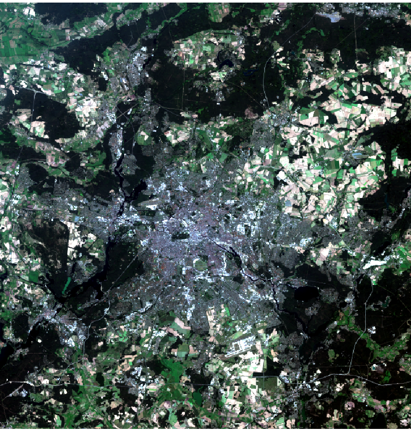
Let's start by making a Natural Color RGB composite from S2 bands: 4,3,2.

```{r P8_plot_rgb_S2, fig.height=5.25, fig.width=5, echo=TRUE, eval=FALSE}

plotRGB(rst, r=3, g=2, b=1, scale=1E5, stretch="lin")

```

![](https://raw.githubusercontent.com/joaofgoncalves/R_exercises_raster_tutorial/master/img/P8_plot_rgb_S2-1.png)


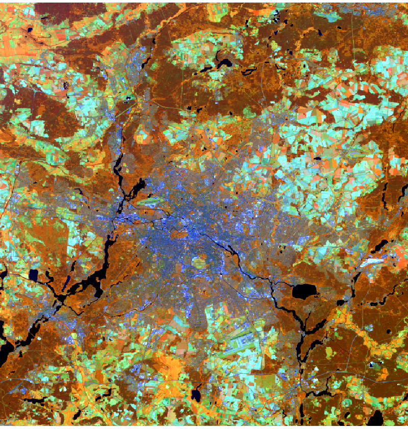
Next, let's see an Healthy vegetation composite from S2 bands: 8,11,2.

```{r P8_plot_b8_b11_b2_S2, fig.height=5.25, fig.width=5, echo=TRUE, eval=FALSE}

plotRGB(rst, r=7, g=9, b=1, scale=1E5, stretch="lin")

```

![](https://raw.githubusercontent.com/joaofgoncalves/R_exercises_raster_tutorial/master/img/P8_plot_b8_b11_b2_S2-1.png)


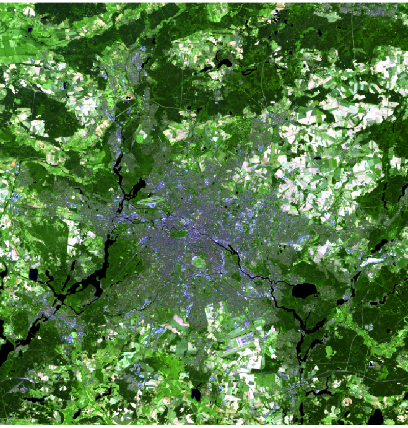
Finally a false color urban using S2 bands: 12,11,4.

```{r P8_plot_b12_b11_b4_S2, fig.height=5.25, fig.width=5, echo=TRUE, eval=FALSE}

plotRGB(rst, r=10, g=9, b=3, scale=1E5, stretch="lin")

```

![](https://raw.githubusercontent.com/joaofgoncalves/R_exercises_raster_tutorial/master/img/P8_plot_b12_b11_b4_S2-1.png)


Now, let's load the training samples used in calibration. These data serves as a reference or 
examples from which the classifier algorithm will "learn" the spectral signatures of each class. 

```{r P8_load_train_data, echo=TRUE, eval=FALSE}

rstTrain <- raster("./data-raw/berlin/train/berlin_lcz_GT.tif")

# Remove zeros from the train set (background NA)
rstTrain[rstTrain==0] <- NA

# Convert the data to factor/discrete representation
rstTrain <- ratify(rstTrain)

# Change the layer name
names(rstTrain) <- "trainClass"

# Visualize the data
plot(rstTrain, main="Train areas by class for Berlin")


```

![](https://raw.githubusercontent.com/joaofgoncalves/R_exercises_raster_tutorial/master/img/P8_load_train_data-1.png)


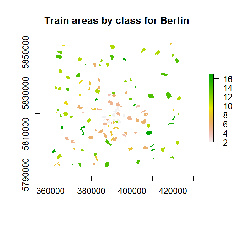
Let's see how many training pixels do we have for each of the 12 classes ($N_{total} = 24537$):

```{r P8_train_data_frequency}

tab <- table(values(rstTrain))
print(tab)

```


Although perhaps not the best approach in some cases, we will convert our raster dataset 
into a `data.frame` object so we can use the RF classifier. Take into consideration, that 
in some cases, depending on the size of your `RasterStack` and the available memory, 
using this approach will not be possible. One simple way to overcome this, would be to convert the training 
raster into a `SpatialPoints` object and then run the function `extract`. This way, only specific 
pixels from the stack are retrieved. In any case, let's proceed to get pixel values into our 
calibration data frame:

```{r P8_load_data_pixel_values, echo=TRUE, eval=FALSE}

rstDF <- na.omit(values(stack(rstTrain, rst)))
rstDF[,"trainClass"] <- as.factor(as.character(rstDF[,"trainClass"]))

```


As you probably noticed from the code above, `NA`'s were removed and the reference class column 
was converted to a categorical/factor variable. In practice, by "removing `NA`'s", it means that 
we are restricting the data only to the set of training pixels in `rstTrain` (reducing from 
428238 to 24537 rows `r emo::ji("thumbsup")`).     

Next up, setting some parameters. In the example, we will use holdout cross-validation (HOCV) to evaluate 
the RF classifier performance. This means that we will use an iterative split set approach, with a training and 
a testing set. So, for this purpose, we need to define the proportion of instances for training (`pTrain`); 
the remaining will be set aside for evaluation. Here I took into consideration the fact that RF tends to take 
some time to calibrate with large numbers of observations (~ >10000) hence the relatively 'large' train proportion. 
We also need to define the number of repetitions in HOCV (`nEvalRounds`).

```{r P8_set_params, echo=TRUE, eval=FALSE}

# Number of holdout evaluation rounds
nEvalRounds <- 20

# Proportion of the data used for training the classifier
pTrain <- 0.5

```

Now let's initialize some objects that will allow us to store some info on the 
the classification performance and validation:


```{r P8_init_objects, echo=TRUE, eval=FALSE}

n <- nrow(rstDF)
nClasses <- length(unique(rstDF[,"trainClass"]))


# Initialize objects

confMats <- array(NA, dim = c(nClasses,nClasses,nEvalRounds))

evalMatrix<-matrix(NA, nrow=nEvalRounds, ncol=3, 
                   dimnames=list(paste("R_",1:nEvalRounds,sep=""), 
                                 c("Accuracy","Kappa","PSS")))

pb <- txtProgressBar(1, nEvalRounds, style = 3)


```

Now, with all set, let´s calibrate and evaluate our RF classifier (use comments to guide 
you through the code):

```{r P8_calibrate_eval_RF, echo=TRUE, eval=FALSE}

# Evaluation function
source(url("https://raw.githubusercontent.com/joaofgoncalves/Evaluation/master/eval.R"))


# Run the classifier

for(i in 1:nEvalRounds){
  
  # Create the random index for row selection at each round
  sampIdx <- sample(1:n, size = round(n*pTrain))

  # Calibrate the RF classifier
  rf <- randomForest(y = rstDF[sampIdx, "trainClass"], 
                     x = rstDF[sampIdx, -1], 
                     ntree = 200)

  # Predict the class to the test set
  testSetPred <- predict(rf, newdata = rstDF[-sampIdx,], type = "response")

  # Get the observed class vector
  testSetObs <- rstDF[-sampIdx,"trainClass"]
  
  # Evaluate 
  evalData <- Evaluate(testSetObs, testSetPred)
  
  evalMatrix[i,] <- c(evalData$Metrics["Accuracy",1],
                      evalData$Metrics["Kappa",1],
                      evalData$Metrics["PSS",1])
  
  # Store the confusion matrices by eval round
  confMats[,,i] <- evalData$ConfusionMatrix
  
  # Classify the whole image with raster::predict function
  rstPredClassTMP <- predict(rst, model = rf, 
                             factors = levels(rstDF[,"trainClass"]))
  
  if(i==1){
    # Initiate the predicted raster
    rstPredClass <- rstPredClassTMP
    
    # Get precision and recall for each class
    Precision <- evalData$Metrics["Precision",,drop=FALSE]
    Recall <- evalData$Metrics["Recall",,drop=FALSE]
    
  }else{
    # Stack the predicted rasters
    rstPredClass <- stack(rstPredClass, rstPredClassTMP)
    
    # Get precision and recall for each class
    Precision <- rbind(Precision,evalData$Metrics["Precision",,drop=FALSE])
    Recall <- rbind(Recall,evalData$Metrics["Recall",,drop=FALSE])
  }
  
  setTxtProgressBar(pb,i)
  
}

# save.image(file = "./data-raw/P8-session.RData")


```

Three classification evaluation measures will be used: (i) __overall accuracy__, (ii) __Kappa__, and,
(iii) __Peirce-skill score__ (PSS; aka true-skill statistic). Let's print out the results by round:

```{r P8_print_eval_matrix}

knitr::kable(evalMatrix, digits = 3)

```

Next, calculate some average and sd measures across all rounds:

```{r}

round(apply(evalMatrix,2,FUN = function(x,...) c(mean(x,...), sd(x,...))), 3)

```

Overall measures seem to indicate that results are acceptable with very low 
variation between calibration rounds. Let's check out some average __precision__ (aka positive predictive value, 
PPV), __recall__ (aka true positive rate, TPR) and F1 measures by class: 

```{r P8_precision_recall_average}

avgPrecision <- apply(Precision,2,mean)
print(round(avgPrecision, 3))


avgRecall <- apply(Recall,2,mean)
print(round(avgRecall, 3))


avgF1 <- (2 * avgPrecision * avgRecall) / (avgPrecision+avgRecall)
print(round(avgF1, 3))

```

Well, things are not so great here... `r emo::ji("sad")` Some classes, such as 4, 9, 5 (different artificial/urban 
types) and 16 (bare soil/sand) are not great. This may be a consequence of the loss of information detail 
due to the 100m re-sampling or some class intermixing, and train data generalization... `r emo::ji("thinking")` ... 
this requires more investigation `r emo::ji("wink")`    

Now let's check the confusion matrix for the best round:

```{r P8_get_conf_matrix}

# Best round for Kappa
evalMatrix[which.max(evalMatrix[,"Kappa"]), , drop=FALSE]

# Show confusion matrix for the best kappa
cm <- as.data.frame(confMats[,,which.max(evalMatrix[,"Kappa"])])

# Change row/col names
colnames(cm) <- rownames(cm) <- paste("c",levels(rstDF[,"trainClass"]),sep="_")

knitr::kable(cm)

```

Since we obtained one classified map for each round we can pull all that 
information by ensembling it together through a majority vote (i.e., calculating the 
modal class). The `raster` package `modal` function makes it really easy to calculate this:

```{r P8_modal_freq_rst, echo=TRUE, eval=FALSE}

rstModalClass <- modal(rstPredClass)

rstModalClassFreq <- modal(rstPredClass, freq=TRUE)

medFreq <- zonal(rstModalClassFreq, rstTrain, fun=median)

```

Using the modal frequency of the 20 classification rounds, let's check out which 
classes obtained the highest 'uncertainty':

```{r P8_show_model_results_freq}

colnames(medFreq) <- c("ClassCode","MedianModalFrequency")

medFreq[order(medFreq[,2],decreasing = TRUE),]

```

These results somewhat confirm those of the class-wise precision/recall. Classes most often shifting 
(lower frequency) are those with lower values for these performance measures.    

Finally, let's plot our results of the the final modal classification map (and modal frequency):

```{r P8_plot_results, fig.width=7, echo=TRUE, eval=FALSE}


par(mfrow=c(1,2), cex.main=0.8, cex.axis=0.8)

plot(rstModalClass, main = "RF modal land cover class")
plot(rstModalClassFreq, main = "Modal frequency")

```

![](https://raw.githubusercontent.com/joaofgoncalves/R_exercises_raster_tutorial/master/img/P8_plot_results-1.png)

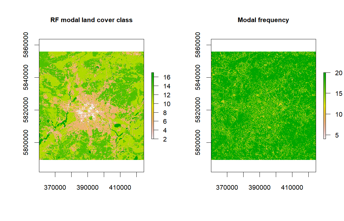
The map on the right provides some insight to identify areas that are more problematic 
for the classification process. However, as you can see, the results are acceptable but 
improvable in many ways.

This concludes our exploration of the raster package and supervised classification for 
this post. Hope you find it useful! `r emo::ji("smile")` `r emo::ji("thumbsup")` `r emo::ji("thumbsup")`