Dashtable is a very important data structure in Dragonfly. This document explains how it fits inside the engine.
Each selectable database holds a primary dashtable that contains all its entries. Another instance of Dashtable holds an optional expiry information, for keys that have TTL expiry on them. Dashtable is equivalent to Redis dictionary but have some wonderful properties that make Dragonfly memory efficient in various situations.

“All problems in computer science can be solved by another level of indirection”
This section is a brief refresher of how redis dictionary (RD) is implemented. We shamelessly "borrowed" a diagram from this blogpost, so if you want a deep-dive, you can read the original article.
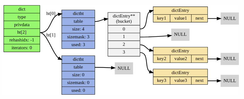
Each RD is in fact two hash-tables (see ht field in the diagram below). The second instance is used for incremental resizes of the dictionary.
Each hash-table dictht is implemented as a classic hashtable with separate chaining. dictEntry is the link-list entry that wraps each key/value pair inside the table. Each dictEntry has three pointers and takes up 24 bytes of space. The bucket array of dictht is resized at powers of two, so usually its utilization is in [50, 100] range.
Let's estimate the overhead of dictht table inside RD.
Case 1: it has N items at 100% load factor, in other words, buckets count equals to number of items. Each bucket holds a pointer to dictEntry, i.e. it's 8 bytes. In total we need:
Case 2: N items at 75% load factor, in other words, the number of buckets is 1.33 higher than number of items. In total we need:
Case 3: N items at 50% load factor, say right after table growth. Number of buckets is twice the number of items, hence we need
In best possible case we need at least 16 bytes to store key/value pair into the table, therefore
the overhead of dictht is on average about 16-24 bytes per item.
Now lets take incremental growth into account. When ht[0] is full (i.e. RD needs to migrate data to a bigger table), it will instantiate a second temporary instance ht[1] that will hold additional 2*N buckets. Both instances will live in parallel until all data is migrated to ht[1] and then ht[0] bucket array will be deleted. All this complexity is hidden from a user by well engineered API of RD. Lets combine case 3 and case 1 to analyze memory spike at this point: ht[0] holds N items and it is fully utilized. ht[1] is allocated with 2N buckets.
Overall, the memory needed during the spike is
To summarize, RD requires between 16-32 bytes overhead.
Dashtable is an evolution of an algorithm from 1979 called extendible hashing.
Similarly to a classic hashtable, dashtable (DT) also holds an array of pointers at front. However, unlike with classic tables, it points to segments and not to linked lists of items. Each segment is, in fact, a mini-hashtable of constant size. The front array of pointers to segments is called directory. Similarly to a classic table, when an item is inserted into a DT, it first determines the destination segment based on item's hashvalue. The segment is implemented as a hashtable with open-addressed hashing scheme and as I said - constant in size. Once segment is determined, the item inserted into one of its buckets. If an item was successfully inserted, we finished, otherwise, the segment is "full" and needs splitting. The DT splits the contents of a full segment in two segments, and the additional segment is added to the directory. Then it tries to reinsert the item again. To summarize, the classic chaining hash-table is built upon a dynamic array of linked-lists while dashtable is more like a dynamic array of flat hash-tables of constant size.

In the diagram above you can see how dashtable looks like. Each segment is comprised of K buckets. For example, in our implementation a dashtable has 60 buckets per segment (it's a compile-time parameter that can be configured).
Below you can see the diagram of a segment. It comprised of regular buckets and stash buckets. Each bucket has k slots and each slot can host a key-value record.

In our implementation, each segment has 56 regular buckets, 4 stash buckets and each bucket contains 14 slots. Overall, each dashtable segment has capacity to host 840 records. When an item is inserted into a segment, DT first determines its home bucket based on item's hash value. The home bucket is one of 56 regular buckets that reside in the table. Each bucket has 14 available slots and the item can reside in any free slot. If the home bucket is full, then DT tries to insert to the regular bucket on the right. And if that bucket is also full, it tries to insert into one of 4 stash buckets. These are kept deliberately aside to gather spillovers from the regular buckets. The segment is "full" when the insertion fails, i.e. the home bucket and the neighbour bucket and all 4 stash buckets are full. Please note that segment is not necessary at full capacity, it can be that other buckets are not yet full, but unfortunately, that item can go only into these 6 buckets, so the segment contents must be split. In case of split event, DT creates a new segment, adds it to the directory and the items from the old segment partly moved to the new one, and partly rebalanced within the old one. Only two segments are touched during the split event.
Now we can explain why seemingly similar data-structure has an advantage over a classic hashtable in terms of memory and cpu.
-
Memory: we need
~N/840entries or8N/840bytes in dashtable directory to host N items on average. Basically, the overhead of directory almost disappears in DT. Say for 1M items we will need ~1200 segments or 9600 bytes for the main array. That's in contrast to RD where we will need a solid8Nbucket array overhead - no matter what. For 1M items, it will obviously be 8MB. In addition, dash segments use open addressing collision scheme with probing, that means that they do not need anything likedictEntry. Dashtable uses lots of tricks to make its own metadata small. In our implementation, the averagetaxper entry is short of 20 bits compared to 64 bits in RD (dictEntry.next). In addition, DT incremental resize does not allocate a bigger table - instead it adds a single segment per split event. Assuming that key/pair entry is two 8 byte pointers like in RD, then DT requires$16N + (8N/840) + 2.5N + O(1) \approx 19N$ bytes at 100% utilization. This number is very close to the optimum of 16 bytes. In unlikely case when all segments just doubled in size, i.e. DT is at 50% of utilization we may need$38N$ bytes per item. In practice, each segment grows independently from others, so the table has smooth memory usage of 22-32 bytes per item or 6-16 bytes overhead. -
Speed: RD requires an allocation for dictEntry per insertion and deallocation per deletion. In addition, RD uses chaining, which is cache unfriendly on modern hardware. There is a consensus in engineering and research communities that classic chaining schemes are slower than open addressing alternatives. Having said that, DT also needs to go through a single level of indirection when fetching a segment pointer. However, DT's directory size is relatively small: in the example above, all 9K could resize in L1 cache. Once the segment is determined, the rest of the insertion, however, is very fast an mostly operates on 1-3 memory cache lines. Finally, during resizes, RD requires to allocate a bucket array of size
2N. That could be time consuming - imagine an allocation of 100M buckets for example. DT on the other hand requires an allocation of constant size per new segment. DT is faster and what's more important - it's incremental ability is better. It eliminates latency spikes and reduces tail latency of the operations above.
Please note that with all efficiency of Dashtable, it can not decrease drastically the overall memory usage. Its primary goal is to reduce waste around dictionary management.
Having said that, by reducing metadata waste we could insert dragonfly-specific attributes into a table's metadata in order to implement other intelligent algorithms like forkless save. This is where some of the Dragonfly's disrupting qualities can be seen.
There are many other improvements in dragonfly that save memory besides DT. I will not be able to cover them all here. The results below show the final result as of May 2022.
To compare RD vs DT I often use an internal debugging command "debug populate" that quickly fills both datastores with data. It just saves time and gives more consistent results compared to memtier_benchmark. It also shows the raw speed at which each dictionary gets filled without intermediary factors like networking, parsing etc. I deliberately fill datasets with a small data to show how overhead of metadata differs between two data structures.
I run "debug populate 20000000" (20M) on both engines on my home machine "AMD Ryzen 5 3400G with 8 cores".
| Dragonfly | Redis 6 | |
|---|---|---|
| Time | 10.8s | 16.0s |
| Memory used | 1GB | 1.73G |
When looking at Redis6 "info memory" stats, you can see that used_memory_overhead field equals
to 1.0GB. That means that out of 1.73GB bytes allocated, a whooping 1.0GB is used for
the metadata. For small data use-cases the cost of metadata in Redis is larger than the data itself.
Now I run Dragonfly on all 8 cores. Redis has the same results, of course.
| Dragonfly | Redis 6 | |
|---|---|---|
| Time | 2.43s | 16.0s |
| Memory used | 896MB | 1.73G |
Due to shared-nothing architecture, Dragonfly maintains a dashtable per thread with its own slice of data. Each thread fills 1/8th of 20M range it owns - and it much faster, almost 8 times faster. You can see that the total usage is even smaller, because now we maintain smaller tables in each thread (it's not always the case though - we could get slightly worse memory usage than with single-threaded case, depends where we stand compared to hash table utilization).
This example shows how much memory Dragonfly uses during BGSAVE under load compared to Redis. Btw, BGSAVE and SAVE in Dragonfly is the same procedure because it's implemented using fully asynchronous algorithm that maintains point-in-time snapshot guarantees.
This test consists of 3 steps:
- Execute
debug populate 5000000 key 1024command on both servers to quickly fill them up with ~5GB of data. - Run
memtier_benchmark --ratio 1:0 -n 600000 --threads=2 -c 20 --distinct-client-seed --key-prefix="key:" --hide-histogram --key-maximum=5000000 -d 1024command in order to send constant update traffic. This traffic should not affect substantially the memory usage of both servers. - Finally, run
bgsaveon both servers while measuring their memory.
It's very hard, technically to measure exact memory usage of Redis during BGSAVE because it creates a child process that shares its parent memory in-part. We chose cgroupsv2 as a tool to measure the memory. We put each server into a separate cgroup and we sampled memory.current attribute for each cgroup. Since a forked Redis process inherits the cgroup of the parent, we get an accurate estimation of their total memory usage. Although we did not need this for Dragonfly we applied the same approach for consistency.

As you can see on the graph, Redis uses 50% more memory even before BGSAVE starts. Around second 14, BGSAVE kicks off on both servers. Visually you can not see this event on Dragonfly graph, but it's seen very well on Redis graph. It took just few seconds for Dragonfly to finish its snapshot (again, not possible to see) and around second 20 Dragonfly is already behind BGSAVE. You can see a distinguishable cliff at second 39 where Redis finishes its snapshot, reaching almost x3 times more memory usage at peak.
Efficient Expiry is very important for many scenarios. See, for example, Pelikan paper'21. Twitter team says that their memory footprint could be reduced by as much as by 60% by employing better expiry methodology. The authors of the post above show pros and cons of expiration methods in the table below:

They argue that proactive expiration is very important for timely deletion of expired items. Dragonfly, employs its own intelligent garbage collection procedure. By leveraging DashTable compartmentalized structure it can actually employ a very efficient passive expiry algorithm with low CPU overhead. Our passive procedure is complimented with proactive gradual scanning of the table in background.
The procedure is a follows:
A dashtable grows when its segment becomes full during the insertion and needs to be split.
This is a convenient point to perform garbage collection, but only for that segment.
We scan its buckets for the expired items. If we delete some of them, we may avoid growing the table altogether! The cost of scanning the segment before potential split is no more the
split itself so can be estimated as O(1).
We use memtier_benchmark for the experiment to demonstrate Dragonfly vs Redis expiry efficiency.
We run locally the following command:
memtier_benchmark --ratio 1:0 -n 600000 --threads=2 -c 20 --distinct-client-seed \
   --key-prefix="key:"  --hide-histogram --expiry-range=30-30 --key-maximum=100000000 -d 256
We load larger values (256 bytes) to reduce the impact of metadata savings of Dragonfly.
| Dragonfly | Redis 6 | |
|---|---|---|
| Memory peak usage | 1.45GB | 1.95GB |
| Avg SET qps | 131K | 100K |
Please note that Redis could sustain 30% less qps. That means that the optimal working sets for Dragonfly and Redis are different - the former needed to host at least 20s*131k items
at any point of time and the latter only needed to keep 20s*100K items.
So for 30% bigger working set Dragonfly needed 25% less memory at peak.
*Please ignore the performance advantage of Dragonfly over Redis in this test - it has no meaning. I run it locally on my machine and it does not represent a real throughput benchmark.
All diagrams in this doc are created in drawio app.