| jupytext | kernelspec | ||||||||||||||||||
|---|---|---|---|---|---|---|---|---|---|---|---|---|---|---|---|---|---|---|---|
|
|
Solving steady-state one-dimensional differential equations with the finite difference approximations.
This Module is focused on solving engineering problems where the governing differential equations are across space and time. The general form of these differential equations are Partial Differential Equations (check out the 3Blue1Brown video). A partial differential equation (PDE) relates the derivatives in space and time. The main difference between ordinary and partial differential equations (ODEs and PDEs) is that ODEs only have one indendent variable e.g. all derivatives are
-
Conductive heat transfer
$q(x,y,t)+\rho C_{p}\frac{\partial T}{\partial t} = -\kappa \nabla^2T$ -
Kirchoff plate mechanics
$D\nabla^2 \nabla^2 w(x,y) = -q(x,y,t)-2\rho h \frac{\partial w^2}{\partial t^2}$ -
Euler Beam mechanics
$EI \frac{\partial^4 w}{\partial x^4} = -\mu \frac{\partial^2 w}{\partial t^2}+q(x,t)$ -
Elastica Buckling equation
$EI\frac{d^2y}{dx^2}=-Py$ - ...
What other PDE equations describe engineering problems?
You can start your discussion of these differential equations with the steady-state solutions along one axis. These analyses include static deflection and buckling of beams and steady-state temperature through a pipe or heat fin.
-
Steady-state Temperature:
$-\kappa A \frac{d^2T}{dx^2}=Q(x)$ -
Static beam deflection: $EI \frac{\partial^4 w}{\partial x^4} = q(x)$
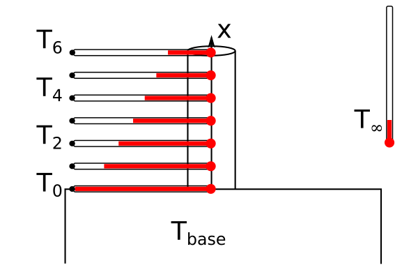
Consider the heat fin shown above, a hot substrate is at temperature
Here is what you do know:
Equations:
where , R is the radius of the cylinderical fin,
Boundary Conditions:
The base of the fin is the same temperature as the base,
The tip of the fin has the same convective heat transfer as the rest of the fin, so the energy conducted to the tip has to be removed through convection,
-
$T_{0} = T_{base}$ -
$T_7=\frac{-h\Delta x}{k}(T_{6}-T_{\infty})+T_5$
If you divide the fin into 6 equally spaced sections, you have 6 equations with 6 unknown temperatures based upon finite difference equations as such,
-
$T_0-2T_1+T_2+\Delta x^2 h'(T_{\infty}-T_1) = 0$ -
$T_1-2T_2+T_3+\Delta x^2 h'(T_{\infty}-T_2) = 0$ -
$T_2-2T_3+T_3+\Delta x^2 h'(T_{\infty}-T_3) = 0$ -
$T_3-2T_4+T_4+\Delta x^2 h'(T_{\infty}-T_4) = 0$ -
$T_4-2T_5+T_5+\Delta x^2 h'(T_{\infty}-T_5) = 0$ -
$T_5-2T_6+T_7+\Delta x^2 h'(T_{\infty}-T_6) = 0 \leftarrow T_7 = \frac{-h\Delta x}{k}(T_{6}-T_{\infty})+T_5$
where andT_{7}.$ You can plug in constants for forced air convection, $h=100W/m^2K$, aluminum fin, $\kappa=200W/mK$, and 60-mm-long and 1-mm-radius fin, the air is room temperature,
import numpy as np
import matplotlib.pyplot as plt
plt.rcParams.update({'font.size': 22})
plt.rcParams['lines.linewidth'] = 3
h=100 # W/m/m/K
k=200 # W/m/K
R=1E-3# radius in m
L=60E-3# length in m
$\left[\begin{array}{cccccc} 2.1 & -1 & 0 & 0 & 0 & 0 \ -1 & 2.1 & -1 & 0 & 0 & 0 \ 0 & -1 & 2.1 & -1 & 0 & 0 \ 0 & 0 & -1 & 2.1 & -1 & 0 \ 0 & 0 & 0 & -1 & 2.1 & -1 \ 0 & 0 & 0 & 0 & -2 & 2.105 \ \end{array}\right] \left[\begin{array}{c} T_{1}\ T_{2}\ T_{3}\ T_{4}\ T_{5}\ T_{6}\end{array}\right]= \left[\begin{array}{c} 10+T_0\ 10\ 10\ 10\ 10\ 10+h\Delta x/k T_{\infty}\ \end{array}\right]$
hp = 2*h/k/R
N=6
dx=L/N

print('h\' = {}, and step size dx= {}'.format(hp,dx))
diag_factor=2+hp*dx**2 # diagonal multiplying factor
print(diag_factor)
Tinfty=20
T0 = 100

A = np.diag(np.ones(N)*diag_factor)-np.diag(np.ones(N-1),-1)-np.diag(np.ones(N-1),1)
A[-1,-2]+= -1
A[-1,-1]+= h/k*dx
b = np.ones(N)*hp*Tinfty*dx**2
b[0]+=T0
b[-1]+=h*dx/k*(Tinfty)
print('finite difference A:\n------------------')
print(A)
print('\nfinite difference b:\n------------------')
print(b)
T=np.linalg.solve(A,b)
print('\nfinite difference solution T(x):\n------------------')
print(T)
print('\nfinite difference solution at x (mm)=\n------------------')
print(np.arange(1,7)*dx*1000)
The equations and solution are shown above for the finite difference set of six coupled linear equations. You solved for the solutions of temperature at $x=[10,~20,~30,~40,~50,60]mm$, then you would exclude that point as well.mm$. We didn't include a solution for $x=0mm$ because it was included in your boundary conditions. If you specified the temperature at
$x=60
When you approximate a derivative as
Below, lets compare your solution to the analytical solution for a fin with the same boundary conditions
L=60e-3
s=np.sqrt(hp)
F=lambda x: 20+80*(np.cosh(s*L-s*x)+h/s/k*np.sinh(s*L-s*x))/(np.cosh(s*L)+h/s/k*np.sinh(s*L))
x=np.arange(0,N+1)*dx
plt.plot(x*1000,F(x),label='analytical')#a*np.cosh(s*x)+b*np.sinh(s*x))
plt.plot(x[1:]*1000,T,'ro',label='finite difference')
plt.plot(x[0],100,'rs',label='base temperature')
plt.xlabel('distance along fin (mm)')
plt.ylabel('Temperature (C)')
plt.legend(bbox_to_anchor=(1,0.5),loc='center left');
Decrease mm$ to $5mm$.
a. Make a plot of the Temperature along the fin.
b. Plot the heat flux through the fin
In the Module 04 project, you solved a finite element analysis problem with stretching beams. A beam is very stiff in tension and compression, but it is usually much less stiff if bent. The Euler-Bernoulli beam theory relates the static deflection of a beam,
If
where $A,~B,~C,andD$ are integration constants. You have four unknowns, so you need four boundary conditions.
Let's consider the simply supported beam with a uniform load. You are considering linear beam mechanics, so you have an underlying assumption that the tension in the beam is negligible. The loads and boundary constraints are shown at the top of the figure below.

solving for A, B, C, and D there results
but you can use the same finite difference method you used above to solve for the deflection
- $L=1
m$ * $E=200e9Pa$ * $I=\frac{0.01^4}{12}m^4$ * $q=100N/m$
Finite difference equation dividing bar length
$\frac{d^4w}{dx^4} \approx \frac{w(x_{i+2})−4w(x_{i+1})+6w(x_i)−4w(x_{i-1})+w(x_{i-2})}{h^4}=\frac{q}{EI}.$
-
$w_{-1} - 4w_0 +6w_1-4w_2+w_3 =\frac{q}{EI}h^4$ -
$w_{0} - 4w_1 +6w_2-4w_3+w_4 =\frac{q}{EI}h^4$ -
$w_{1} - 4w_2 +6w_3-4w_4+w_5 =\frac{q}{EI}h^4$ -
$w_{2} - 4w_3 +6w_4-4w_5+w_6 =\frac{q}{EI}h^4$ -
$w_{3} - 4w_4 +6w_5-4w_6+w_7 =\frac{q}{EI}h^4$
Boundary Conditions:
$w(0)=0=w_0$ $w(L)=0=w_6$ $w''(0)=0=\frac{w_{-1}-2w_{0}+w_{1}}{h^2} \rightarrow w_{-1}=-w_{1}$ $w''(L)=0=\frac{w_{5}-2w_{6}+w_{7}}{h^2} \rightarrow w_{7}=-w_{5}$
Final linear equation set:
-
$5w_1-4w_2+w_3 =\frac{q}{EI}h^4$ -
$-4w_1 +6w_2-4w_3+w_4 =\frac{q}{EI}h^4$ -
$w_{1} - 4w_2 +6w_3-4w_4+w_5 =\frac{q}{EI}h^4$ -
$w_{2} - 4w_3 +6w_4-4w_5+w_6 =\frac{q}{EI}h^4$ -
$w_{3} - 4w_4 +5w_5-4w_6 =\frac{q}{EI}h^4$
$\left[\begin{array}{cccccc} 5 & -4 & 1 & 0 & 0 \ -4 & 6 & -4 & 1 & 0 \ 1 & -4 & 6 & -4 & 1 \ 0 & 1 & -4 & 6 & -4 \ 0 & 0 & 1 & -4 & 5 \end{array}\right] \left[\begin{array}{c} w_{1}\ w_{2}\ w_{3}\ w_{4}\ w_{5} \end{array}\right]= \frac{qh^4}{EI}\left[\begin{array}{c} 1\ 1\ 1\ 1\ 1 \end{array}\right]$
L=1
h=L/6
E=200e9
I=0.01**4/12
q=100

A=np.diag(np.ones(5)*6)\
+np.diag(np.ones(4)*-4,-1)\
+np.diag(np.ones(4)*-4,1)\
+np.diag(np.ones(3),-2)\
+np.diag(np.ones(3),2)
A[0,0]+=-1
A[-1,-1]+=-1

b=-np.ones(5)*q/E/I*h**4

w=np.linalg.solve(A,b)
xnum=np.arange(0,L+h/2,h)
print('finite difference A:\n------------------')
print(A)
print('\nfinite difference b:\n------------------')
print(b)
print('\ndeflection of beam (mm)\n-------------\n',w*1000)
print('at position (m) \n-------------\n',xnum[1:-1])
x=np.linspace(0,L)
w_an=-q*x*(L**3-2*x**2*L+x**3)/24/E/I

plt.plot(xnum,np.block([0,w*1000,0]),'s')
plt.plot(x,w_an*1000)
Divide the simply-supported beam into 12 sections and plot the deflection as a function of distance along the beam with a uniform load.
What is the convergence rate for this central difference method? Hint: check the magnitude of round-off error for central difference methods.
- The difference between a PDE and an ODE
- How to approximate differential equations with boundary conditions
- Solve steady-state heat transfer problem
- Solve static deflection of elastic beam
- Demonstrate convergence of finite difference solutions